REVIEW 3 major objections 4 minor 15 references
Targeted Highly Adaptive Lasso Minimum Loss Estimation of Target Functions
T0 review · 3 major / 4 minor · reviewed 2026-07-11 · grok-4.5
Pith's one-line read Targeted HAL-MLE estimates non-pathwise differentiable curves at rates that depend only on the target function's smoothness and dimension.
desk verdict Solid TMLE/HAL construction for non-pathwise functionals with real asymptotic theorems; positivity gap is real but does not erase the contribution. read the letter →
The pith
A machine-rendered reading of the paper's core claim, the machinery that carries it, and where it could break.
The reading
What carries the argument
The pathwise-differentiable projection of the target onto a finite-dimensional k-th order spline working model, followed by a LASSO (or relaxed LASSO) targeting step that solves the efficient influence curve of that projection while controlling the sectional variation norm.
What would settle it
In a simulation where the true dose-response curve belongs to a known k-th order smoothness class, check whether the Monte-Carlo pointwise RMSE of Targeted HAL-MLE scales like n to the power -k*/(2k*+1) (up to log factors) while a non-targeted HAL plug-in scales only with the slower rate of the higher-dimensional outcome regression; failure of that separation would refute the rate claim.
Extended reading notes
Core claim
Targeted HAL-MLE, obtained by projecting a non-pathwise differentiable target onto a large HAL-spline working model and replacing the usual TMLE MLE step with a LASSO over those basis functions, is pointwise asymptotically normal at a rate determined only by the target function's own dimension and smoothness class, not by the ambient dimension of the outcome regression.
Load-bearing premise
The product of the convergence rates of the initial outcome-regression and propensity estimators must be fast enough relative to the working-model size, and the propensity must stay bounded away from zero, so that second-order remainders and empirical-process terms stay negligible after targeting.
Editorial analysis
A structured set of objections, weighed in public.
Referee Report
Summary. The paper develops Targeted HAL-MLE (T-HAL-MLE) for non-pathwise-differentiable functional parameters such as the continuous-exposure dose-response curve. It projects the target function onto a finite-dimensional k-th-order spline working model (making the projection pathwise differentiable), then runs a TMLE whose targeting step is replaced by an L1-penalized LASSO over a large initial HAL basis. Under a strong positivity bound and a product-rate condition on the initial HAL fits for the outcome regression and propensity, the resulting estimator is shown to be pointwise asymptotically normal at the rate determined solely by the dimension and smoothness of the target function (Theorems 3.4, 4.2, 6.3, 6.5), up to log-n factors. An extensive Monte-Carlo study (3 DGPs × 2 treatment laws × 3 sample sizes × 1000 replications) reports lower bias and RMSE than the plug-in HAL-MLE, together with influence-curve Wald intervals.
Significance. If the asymptotic claims hold under the stated conditions, the work supplies a fully data-adaptive procedure for inference on infinite-dimensional causal functionals that avoids both parametric working models and user-specified sieves, while attaining the minimax rate of the lower-dimensional target rather than that of the high-dimensional outcome regression. The careful first-order expansions, double-robust remainder analysis, and transfer lemmas from fixed to data-adaptive sieves constitute a solid technical contribution; the simulation design is unusually thorough for the area. These features make the paper a useful addition to the TMLE/HAL literature on continuous exposures, provided the gap between the strong positivity assumption and realistic continuous-treatment regimes is closed or clearly delimited.
major comments (3)
- [Theorem 3.4 / Section 7 / Figures 3–5,7] Theorems 3.4, 4.2, 6.3 and 6.5 all invoke the uniform positivity bound min_a g0(a|W)>δ>0 (and the same bound for gn) to guarantee that the second-order remainder R_Ψλ,a = O(∥g-g0∥_∞ ∥Q̄n-Q̄0∥_∞ n(λ)) and the entropy-integral empirical-process term remain o_P of the target rate (n(λ)/n)^{1/2}. Under the normal treatment law of Section 7 the density of A decays in the tails of [0,10], so the bound fails on a set of positive measure. Precisely those tails produce the residual bias, inflated bias/MC-SE ratios and Wald under-coverage documented in Figures 3–5 and 7. The theory therefore does not cover the simulation regime in which practical performance is most questionable; either a weaker positivity analysis or an explicit robustification (Appendix A) must be shown to restore the claimed normality, or the scope of the inference claims must be restricted.
- [Section 5.1 / Section 7.2] The rate-optimal L1-norm selector of Section 5.1 is defined by the free constants c1 and c2 that bound the working-model size between c1 n^{1/(2k*+1)} and c2 n^{1/(2k*+1)}. These constants are chosen post-hoc by a grid search that minimises RMSE on a separate set of simulations (Section 7.2: c1=6, c2=9). Because the asymptotic statements treat n(λ) as given, the finite-sample validity of the normality and coverage claims depends on an unreported tuning step. A data-driven, theoretically justified selector (or a sensitivity analysis over a range of c1,c2) is needed before the method can be regarded as fully automatic.
- [Section 7.2 / Figures 4,7] Wald intervals constructed from the estimated efficient influence curve of the projected parameter substantially undercover under both treatment laws (Figure 7), while the same intervals that use the Monte-Carlo standard deviation achieve near-nominal coverage (Figure 4). The discrepancy indicates that the variance estimator itself is unreliable once the LASSO active set is data-dependent and the Gram matrix is inverted by Moore-Penrose (Section 7.2). The paper mentions targeted bootstrap as a possible remedy but does not implement or analyse it; without a working variance estimator the claim of “inference on functional parameters” remains incomplete.
minor comments (4)
- [Section 2 / Table 1] Notation for the two smoothness indices k (target) and k-bar (outcome regression) is introduced late and occasionally swapped; a single consistent table of symbols at the beginning of Section 2 would help.
- [Algorithm 1] Algorithm 1 is clear, but the closed-form OLS projection step (line 7) is written with Pn of the plug-in marginal; it should be noted that this is an empirical L2 projection onto the selected basis and is therefore itself subject to the same positivity issues as the targeting step.
- [Section 7.4] Figures 1–8 are informative but the box-plot whiskers frequently extend beyond the plotted range; either clip or use a log scale for RMSE under the high-frequency DGP.
- [Introduction] The discussion of related work (i-learner, EP-learner) correctly notes the absence of pointwise normality proofs, yet does not compare finite-sample coverage or computational cost; a short paragraph or table would strengthen the positioning.
Circularity Check
No significant circularity: asymptotic normality is derived from first-order expansions and known HAL rates; the only mild self-reference is the simulation-tuned constants for the L1-norm selector, which do not enter the theorems.
-
self citation load bearing
[Section 5.1 / Simulation Section 7.2]
"The constants c1 = 6 and c2 = 9 were selected by evaluating a grid of candidate values in a separate set of simulations and choosing those that minimized RMSE across settings."
The numerical thresholds that implement the theoretically motivated rate n^{1/(2k*+1)} are chosen by minimizing RMSE on a simulation grid that is not independent of the paper's own evaluation design. This is a minor, non-load-bearing self-reference: the asymptotic theorems themselves only require n(λ)∼n^{1/(2k*+1)} up to log n factors and do not depend on the particular constants 6 and 9.
full rationale
The paper's central claims (Theorems 3.4, 4.2, 6.3, 6.5) are obtained by writing the exact first-order expansion of the pathwise-differentiable projection Ψ_λ, controlling the second-order remainder by the product of nuisance rates of the initial HAL fits, and controlling the empirical-process term by the entropy integral of the HAL function class. These steps rely on standard TMLE arguments and on previously published dimension-free rates for HAL (van der Laan 2023), which are independent of the present target-function results. The projection coefficients α_λ are defined by an L2 minimization that is not fitted to the quantity being predicted; the LASSO targeting step solves a score equation for that projection and does not force the asymptotic normality statement by construction. The only mild self-reference is the choice of numerical constants c1=6, c2=9 that define the rate-optimal L1-norm interval; those constants are selected by a separate simulation grid and affect only finite-sample performance, not the theoretical statements. Consequently the derivation is self-contained against external benchmarks and does not reduce any claimed prediction to a fitted input or to a load-bearing self-citation chain.
Assumptions & free parameters
free parameters (2)
- c1 (lower rate constant for sieve size) =
6
- c2 (upper rate constant for sieve size) =
9
assumptions (5)
- domain assumption k-th order HAL-MLE converges at the dimension-free rate O_+(n^{-k*/(2k*+1)}) in sup-norm when the true function has finite k-th order sectional variation norm.
- domain assumption The L2-projection of any function in D^{(k)}_M onto an n(λ)-dimensional spline working model has uniform approximation error O_+(n(λ)^{-k*}).
- domain assumption Strong positivity: min_a g0(a|W) > δ > 0 almost everywhere.
- domain assumption The product of the HAL rates of the initial outcome and propensity estimators is o of the target rate after multiplication by n(λ).
- standard math Standard empirical-process entropy integrals for classes of bounded sectional variation norm control the remainder terms after normalization by n(λ).
invented entities (1)
-
Targeted HAL-MLE (T-HAL-MLE)
Cite this review
Pith. "Pith review of Targeted Highly Adaptive Lasso Minimum Loss Estimation of Target Functions." pith.science (2026). https://pith.science/paper/KCEH6AEH
@misc{pith2026260703824,
  author       = {Pith},
  title        = {Pith review of: Targeted Highly Adaptive Lasso Minimum Loss Estimation of Target Functions},
  year         = {2026},
  howpublished = {\url{https://pith.science/paper/KCEH6AEH}},
  note         = {Machine review of arXiv:2607.03824}
}
abstract
We propose a Targeted Highly Adaptive Lasso for estimation of non-pathwise differentiable functional parameters such as the dose-response curve (DRC) for continuous exposure. We assume the target function lies in the $k$-th order smoothness class used to define the $k$-th order Highly Adaptive Lasso (HAL), which can be well approximated by linear spans of $k$-th order spline basis functions. We construct a projection of the true target function onto a large finite dimensional working model spanned by an initial set of $k$-th order spline basis functions, which defines a pathwise differentiable approximation of the target functional parameter. A standard TMLE is then applied with a data-adaptive initial fit, replacing the MLE targeting step with a LASSO step over HAL spline basis functions that span the target function. We prove that the resulting Targeted HAL-MLE is pointwise asymptotically normally distributed and achieves a convergence rate determined solely by the dimension and smoothness of the target function, giving dimension free rates up till $\log n$-factors. Through a simulation study for the DRC, we show that the Targeted HAL outperforms a HAL plug-in estimator in terms of bias and mean squared error. Targeted HAL offers a fully data-adaptive approach to inference on functional parameters without requiring sieve specification or parametric assumptions.
Figures


Figures from the paper (14 more)





Reference graph
Works this paper leans on
-
[1]
URLhttps://academic.oup.com/aje/article/191/9/1640/6580570
doi:10.1093/aje/kwac087. URLhttps://academic.oup.com/aje/article/191/9/1640/6580570. Nima S Hejazi, David C Benkeser, and Mark J van der Laan. haldensify: Highly adaptive lasso conditional density estimation. https://github.com/nhejazi/haldensify,
-
[2]
URL https://doi.org/10.5281/zenodo. 3698329. R package version 0.2.5. Jonathan Levy and Mark Laan. Kernel smoothing of the treatment effect cdf, 11
-
[3]
URLhttps://arxiv.org/abs/2506.17214. R. Neugebauer and M. J. van der Laan. Nonparametric causal effects based on marginal structural models.J Stat Plan Infer, 137(2):419–434,
-
[4]
doi:10.1017/S0305004100030401. J.M. Robins, M.A. Hernan, and B. Brumback. Marginal structural models and causal inference in epidemiology. Epidemiol, 11(5):550–560,
-
[5]
doi:10.1007/s10985-022-09576-2
ISSN 1380-7870, 1572-9249. doi:10.1007/s10985-022-09576-2. URLhttps://link.springer.com/10.1007/s10985-022-09576-2. 29 Targeted Highly Adaptive Lasso Minimum Loss Estimation of Target FunctionsA PREPRINT Helene C. W. Rytgaard, Frank Eriksson, and Mark J. Van Der Laan. Estimation of time-specific intervention effects on continuously distributed time-to-eve...
-
[6]
ISSN 0006-341X, 1541-0420. doi:10.1111/biom.13856. URL https://onlinelibrary. wiley.com/doi/10.1111/biom.13856. S. J. Sheather and M. C. Jones. A Reliable Data-Based Bandwidth Selection Method for Kernel Density Estimation. Journal of the Royal Statistical Society: Series B (Methodological), 53(3):683–690, January
-
[7]
doi:10.1111/j.2517-6161.1991.tb01857.x
ISSN 0035-9246. doi:10.1111/j.2517-6161.1991.tb01857.x. Junming Shi, Wenxin Zhang, Alan E. Hubbard, and Mark van der Laan. Hal-based plug-in estimation with pointwise asymptotic normality of the causal dose-response curve,
-
[8]
Lars van der Laan, Marco Carone, and Alex Luedtke. Combining T-learning and DR-learning: A framework for oracle-efficient estimation of causal contrasts.arXiv preprint arXiv:2402.01972,
Show all 15 references
-
[9]
Higher order spline highly adaptive lasso estimators of functional parameters: Pointwise asymptotic normality and uniform convergence rates.arXiv preprint arXiv:2301.13354,
Mark van der Laan. Higher order spline highly adaptive lasso estimators of functional parameters: Pointwise asymptotic normality and uniform convergence rates.arXiv preprint arXiv:2301.13354,
-
[10]
doi:10.1515/jci-2024-0051
ISSN 2193-3685. doi:10.1515/jci-2024-0051. M. P. Wand and M. C. Jones.Kernel Smoothing. Chapman and Hall/CRC, New York, December
2024 doi
-
[11]
doi:10.1201/b14876
ISBN 978-0-429-17059-1. doi:10.1201/b14876. Wenxin Zhang, Junming Shi, Alan Hubbard, and Mark van der Laan. Constructing confidence intervals for infinite- dimensional functional parameters by highly adaptive lasso,
-
[12]
URLhttps://arxiv.org/abs/2507.10511. 30 Targeted Highly Adaptive Lasso Minimum Loss Estimation of Target FunctionsA PREPRINT Single discontinuity Multiple discontinuities High frequency Uniform Treatment DistributionNormal Treatment Distribution 500 1000 2000 500 1000 2000 500...
2000
-
[13]
Each observation is the mean width at one test point
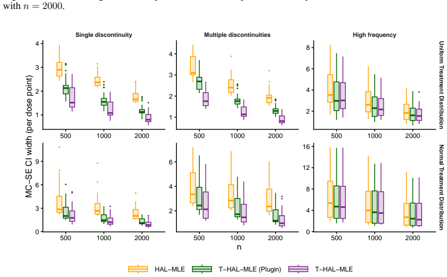
Single discontinuity Multiple discontinuities High frequency Uniform Treatment DistributionNormal Treatment Distribution 500 1000 2000 500 1000 2000 500 1000 2000 500 1000 2000 500 1000 2000 500 1000 2000 2 4 6 8 0 4 8 12 16 1 2 3 4 2 4 6 1 2 3 4 0 3 6 9 n MC−SE CI width (per ...
2000
-
[14]
Here P ∗ n =P ∗ n,λn
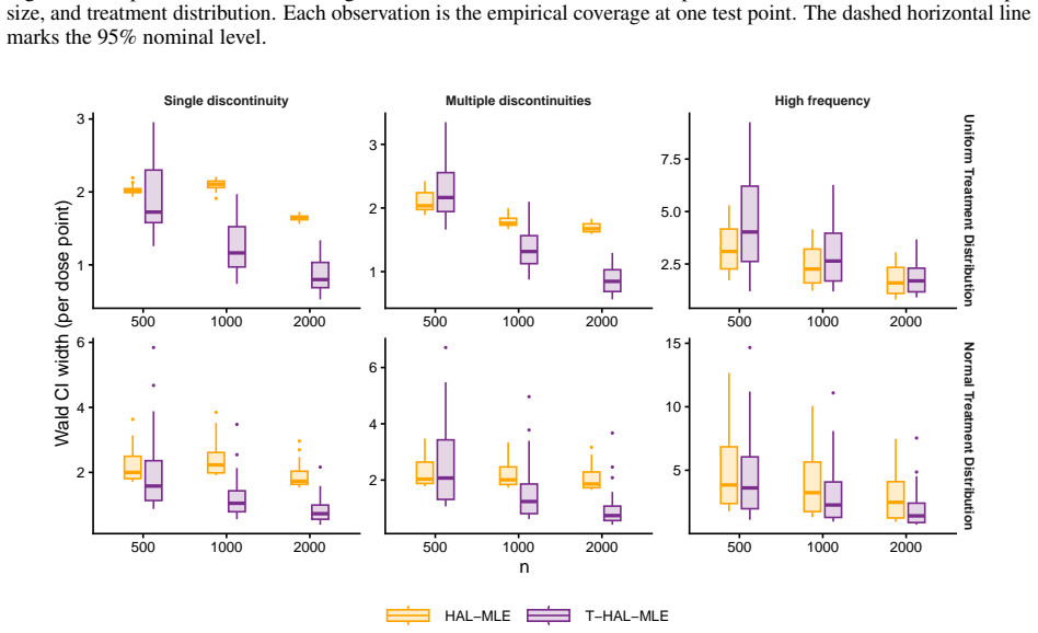
= O+(n(λ)−k∗ 1 )is negligible relative to(n(λ)/n) 1/2 by somelogn-factor then also yields (n/n(λn))1/2(Ψλ(P ∗ n)−Ψ(P 0))(v)/σn(v)⇒ d N(0,1), pointwise for each v, where σ2 n(v) is the sample variance of n(λ)−1/2D∗ Ψλ(),v,P ∗n . Here P ∗ n =P ∗ n,λn. This yields pointwise 0.95-...
2000
-
[15]
Each row corresponds to one outcome distribution
48 Targeted Highly Adaptive Lasso Minimum Loss Estimation of Target FunctionsA PREPRINT n = 500 n = 1000 n = 2000 Single discontinuityMultiple discontinuitiesHigh frequency 2.5 5.0 7.5 2.5 5.0 7.5 2.5 5.0 7.5 2.5 5.0 7.5 2.5 5.0 7.5 2.5 5.0 7.5 2.5 5.0 7.5 2.5 5.0 7.5 2.5 5.0 ...
2000
Reviewed July 11, 2026 · model on record in the stance chip above.
Discussion (0). Sign in to comment.