REVIEW 3 major objections 6 minor 2 cited by
HRMOS: A High-Resolution Multi-Object Spectrograph for the VLT
T0 review · 3 major / 6 minor · reviewed 2026-07-11 · grok-4.5
Pith's one-line read No existing or planned 8 m-class instrument combines multi-object spectroscopy with R=80 000 resolution and 10 m/s radial-velocity stability; HRMOS is designed to fill that gap.
desk verdict Solid VLT 2030 white paper that correctly identifies a real capability gap and backs the science with concrete simulations; the RV budget is the main engineering risk, not a science-case failure. read the letter →
The pith
A machine-rendered reading of the paper's core claim, the machinery that carries it, and where it could break.
The reading
What carries the argument
The baseline HRMOS instrument concept: a hybrid front-end fibre positioner with dual-zone atmospheric dispersion correction, double-scrambling fibre link with image slicers, three VPH-grating spectrograph arms under thermal/pressure control, and simultaneous laser-frequency-comb calibration, sized to meet an RV error budget of roughly 8 m/s total.
What would settle it
On-sky commissioning and stability campaigns that measure the delivered multi-fibre RV floor; if the residual systematic error substantially exceeds the 10 m/s requirement after calibration, the exoplanet-occurrence and precise-kinematics science cases fail as stated.
Extended reading notes
Core claim
The central claim is that a single VLT instrument combining multiplex of 50–60 fibres, resolving power R=80 000, blue coverage to 385 nm, and residual radial-velocity precision of order 10 m/s will enable statistically large, high-fidelity spectroscopic studies in crowded fields that are infeasible with either pure multi-object survey spectrographs or single-object ultra-stable spectrographs alone.
Load-bearing premise
That the hybrid positioner, double scrambling, stabilised spectrographs and simultaneous calibration will actually keep residual radial-velocity systematics at or below about 7 m/s under real Nasmyth operating conditions.
Editorial extensions
If this is right
- Complete surveys of giant-planet occurrence become feasible in open and globular clusters and in bulge and dwarf-galaxy fields with well-known ages and metallicities.
- Nucleocosmochronology ages from Th/Eu (and U) can be averaged over many members of the oldest globular clusters, giving a model-independent lower bound on the age of the Universe.
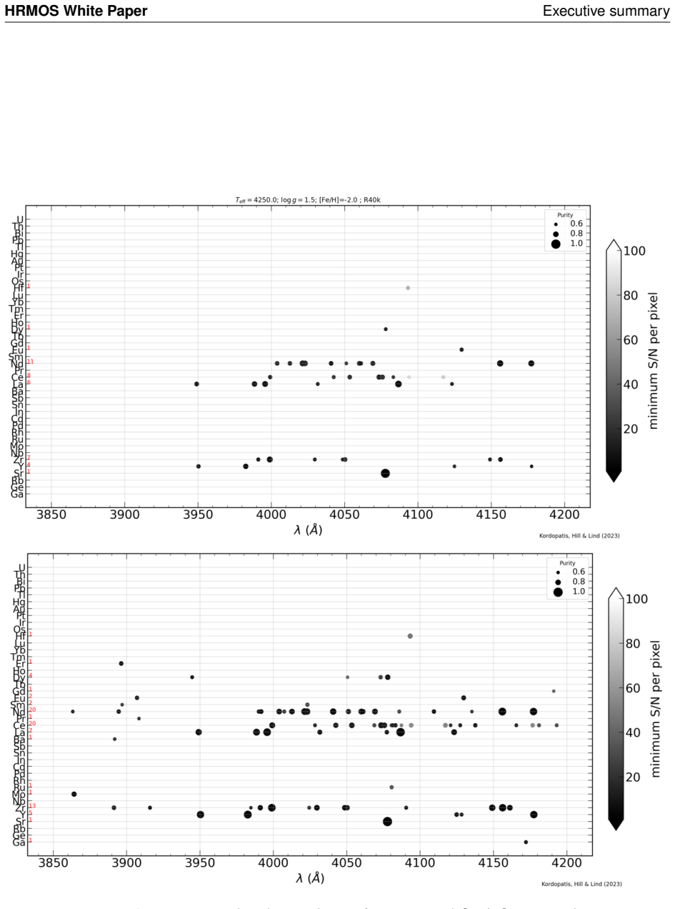
- Full abundance patterns and Ba isotopic fractions for large samples of metal-poor stars and accreted populations can distinguish r-, s- and i-process sites and map hierarchical assembly of the Magellanic Clouds and Sagittarius.
- High-precision light-element and isotopic work (C isotopes, S, Mg isotopes) in coeval cluster stars can calibrate mixing, diffusion and polluter models for multiple populations.
- HRMOS becomes the natural high-resolution bridge between large surveys (4MOST, Gaia, PLATO) and ELT single-object instruments such as ANDES.
Reading between the lines
- If the dual-ADC hybrid architecture works as budgeted, it may become a template for other high-stability multi-object designs that need both crowded-field packing and full optical wavelength coverage.
- Failure to meet the RV floor would still leave a powerful abundance and isotope machine; the white paper’s science portfolio is broader than the exoplanet case alone.
- The explicit coupling of the instrument to laboratory atomic data and 3D non-LTE atmosphere grids implies that first-light science return depends as much on those community deliverables as on hardware.
- A successful HRMOS would pressure future survey facilities to plan explicit high-resolution follow-up pathways rather than treating R~20 000 as the end point.
Editorial analysis
A structured set of objections, weighed in public.
Referee Report
Summary. This White Paper presents the scientific rationale and baseline instrument concept for HRMOS, a proposed VLT Nasmyth multi-object spectrograph combining R=80 000, 50–60 fibres, optical coverage down to ~385 nm, and a radial-velocity precision requirement of 10 m s^{-1} (goal 5 m s^{-1}). It argues that no existing or planned 8 m-class facility offers this combination, and that the design enables statistically significant high-fidelity abundance, isotope, line-profile and RV studies in crowded fields (open/globular clusters, bulge, nearby dwarfs). Science drivers span exoplanet occurrence across environments, nucleosynthesis (C isotopes, S, s/i/r-process and Ba isotopes), hierarchical assembly of MW satellites, nucleocosmochronology (Th/Eu), cluster physics, and ISM/CGM absorption. Technical heritage from FLAMES/MOONS, a dual-zone ADC hybrid positioner, double scrambling, three VPH arms and simultaneous LFC calibration is summarised, with an RV error budget claiming ~8.2 m s^{-1} total residual.
Significance. If the instrument is built and meets its TLRs, it would occupy a genuinely empty region of the MOS–resolution–stability parameter space and provide a natural bridge between 4MOST/Gaia/PLATO-class surveys and ELT/ANDES single-object work. The science cases are unusually well supported for a white paper: concrete RV detectability maps, HRMOS-like spectrum translators from ESPRESSO/HARPS, synthetic spectra for C isotopes, S I Multiplet 8, Ba isotopes, Th/Eu, Mg precision vs SNR, and binary recovery simulations give falsifiable performance targets. Explicit integration of laboratory atomic data and expanded 3D RHD/non-LTE modelling into the project plan is a strength. The document is therefore a credible community input to the VLT 2030 process rather than a pure advocacy brochure.
major comments (3)
- §1.3.8 and Table 1.2 (Eqs. 1.1–1.5): The residual systematic budget of ~6.7 m s^{-1} (total ~8.2 m s^{-1}) is load-bearing for the exoplanet occurrence-rate and precise-kinematics cases (Ch. 2, §6.6). The budget assumes double-scrambling gain ~10^4, ~30% LFC calibration residuals, and thermo-mechanical control at a few mK h^{-1}. Under real VLT Nasmyth thermal/pressure cycles, dual-zone ADC residuals, fibre stress and operational overheads these terms may exceed the allocation. The manuscript should add a short risk/mitigation subsection quantifying which science products survive if residual systematics are 15–20 m s^{-1} rather than ~7 m s^{-1}, and which require the goal 5 m s^{-1}.
- §1.3.3–1.3.4 (hybrid r–θ / pick-and-place dual-ADC architecture): The dual-zone solution (central common ADC for ≥10 arcsec separation; peripheral per-fibre ADCs for ≥30 arcsec) is central to crowded-field science (GC cores, bulge). Technology readiness is asserted by analogy to ESPRESSO/MOONS/KMOS, but no quantitative residual-dispersion or coupling-efficiency budget across the 385–677 nm range is given for the two zones. A table or figure of expected ADC residual vs airmass and zone would make the 10-arcsec inner-field claim more defensible.
- Executive summary and Ch. 8–9: Success of abundance/isotope science is conditioned on laboratory atomic data and expanded 3D RHD + multi-element non-LTE grids being available before first light. This is stated as a proactive project component, but no schedule, resource envelope or success metrics are given. Because several key diagnostics (Th, U, Ba isotopes, weak S I, heavy n-capture lines) are systematics-limited rather than photon-noise-limited, the White Paper should identify which science cases remain robust if only partial atomic/3D grids are delivered by first light.
minor comments (6)
- Fig. 1.6 and 1.7: Symbol sizes and colour coding for multiplex and telescope aperture are useful, but the caption of Fig. 1.7 should state explicitly which instruments are integral-field vs multi-object vs single-object to avoid misreading the crowded legend.
- Table 1.2: Units are listed as cms^{-1} while the text discusses m s^{-1}; the conversion is clear but a consistent unit choice (or dual labelling) would reduce reader friction.
- §2.4.2: The HRMOS-like spectrum translator is a valuable tool; stating whether the code will be public (and under what licence) would strengthen reproducibility claims.
- §3.4.3 / Fig. 3.4: Ba-isotope residual panels are informative; adding the corresponding UVES-like residual amplitude in the same figure (already discussed in text) would make the factor-of-two gain immediately visual.
- Chapter 11 observational strategies are concrete; a single summary table of nights-per-science-case (exoplanets, GCs, LMC/SMC/Sgr, bulge) would help readers and time-allocation committees.
- Acronym list is comprehensive; ensure first use of every acronym in the main text is expanded (a few late-chapter first uses appear only as acronyms).
Circularity Check
No circular derivation: instrument white paper with requirements flowing from science drivers and engineering estimates, not self-referential predictions.
full rationale
HRMOS is a design-and-science-case White Paper, not a first-principles derivation of a physical result. Top-level requirements (R=80 000, RV precision 10 m s^{-1} goal 5 m s^{-1}, 50–60 fibres, coverage to 385 nm; Table 1.1) are stated as design targets motivated by the science chapters; the instrument concept and RV error budget (Section 1.3.8, Table 1.2, Eqs. 1.1–1.5) are engineering estimates under stated assumptions (double scrambling gain ~10^4, LFC calibration residual factor ~3, N_lines ~800, etc.), not parameters fitted to data and then re-presented as independent predictions. Detectability simulations (Ch. 2), abundance/isotope feasibility spectra (Ch. 3–5), and target strategies (Ch. 11) are forward calculations given those design parameters. Self-citations (Magrini et al. 2023 first White Paper, Brucalassi et al. 2022, Riva et al. 2026, workshop presentations) document prior concept development and community process; none supply a uniqueness theorem or load-bearing premise that forces the performance claims. Uniqueness of the R–multiplex niche (Figs. 1.6–1.7) is an external landscape comparison, not a self-referential renaming. No self-definitional loop, fitted-input-as-prediction, or ansatz smuggled via citation reduces a central claim to its inputs by construction. Score 0 is the proportionate finding.
Assumptions & free parameters
free parameters (4)
- Resolving power R =
80000
- RV precision requirement =
10 m s^{-1} (goal 5)
- Multiplex (number of fibres) =
50-60
- Spectral windows (central wavelengths) =
three windows ~385-677 nm
assumptions (5)
- domain assumption No existing or funded 8 m-class instrument combines R≳50 000 with multiplex ≳20 and RV stability ≲10 m s^{-1}.
- domain assumption Double scrambling yields a gain factor ~10^4, reducing guiding-induced RV systematics to sub-cm s^{-1}.
- domain assumption Simultaneous LFC calibration reduces residual systematics by a factor ~3 (30 % residuals).
- domain assumption Science questions listed (nucleocosmochronology ages, cluster exoplanet occurrence, r-process sites, hierarchical assembly of LMC/SMC/Sgr) will remain open and high-priority in the 2030s.
- ad hoc to paper Adequate laboratory atomic data and expanded 3D RHD + multi-element non-LTE grids will be available by first light.
Cite this review
Pith. "Pith review of HRMOS: A High-Resolution Multi-Object Spectrograph for the VLT." pith.science (2026). https://pith.science/paper/2UT3MZSV
@misc{pith2026260704916,
  author       = {Pith},
  title        = {Pith review of: HRMOS: A High-Resolution Multi-Object Spectrograph for the VLT},
  year         = {2026},
  howpublished = {\url{https://pith.science/paper/2UT3MZSV}},
  note         = {Machine review of arXiv:2607.04916}
}
read the original abstract
This White Paper presents the scientific rationale and instrument concept for HRMOS (High-Resolution Multi-Object Spectrograph), a next-generation instrument proposed for the ESO Very Large Telescope within the VLT 2030 roadmap. Current and planned facilities offer either multi-object spectroscopy or ultra-high spectral resolution, but not both. HRMOS fills this gap by combining very high spectral resolution, multi-object capability, and radial-velocity stability, enabling transformative studies in Galactic and extragalactic astrophysics. The baseline design provides a resolving power of R = 80000, radial-velocity precision of 10 m s-1 (goal: 5 m s-1), simultaneous observations of 50-60 targets, and broad optical coverage down to 385 nm. These capabilities enable precise measurements of elemental abundances, isotopic ratios, line profiles, and radial velocities for large stellar samples, including crowded fields, star clusters, the Galactic bulge, and nearby dwarf galaxies. HRMOS will address key questions on the age of the oldest stellar populations through nucleocosmochronology, the formation and survival of planetary systems, the assembly history of the Milky Way and satellites, the origin of the heaviest elements, stellar evolution, and the chemical and dynamical properties of the interstellar and circumgalactic medium. It will bridge large spectroscopic surveys and the next generation of extremely large telescopes, with strong synergies with 4MOST, Gaia, TESS, PLATO, the proposed Haydn mission, and future ELT instruments. Building on VLT/FLAMES heritage, HRMOS represents a strategic investment for European astronomy in the 2030s.
Figures


Figures from the paper (56 more)




Forward citations
Cited by 2 Pith papers
-
HRMOS: a very high-resolution, multi-object spectrograph for the ESO VLT
HRMOS is a proposed VLT instrument combining R=80,000 spectroscopy with 50–60 simultaneous fibers and 10 m/s radial-velocity precision across three optical bands.
-
Stellar Population Astrophysics (SPA) with the TNG. Beyond the iron peak: Galactic evolution of molybdenum, ruthenium and zirconium through open clusters
First large-sample ruthenium abundances in open clusters show Mo and Ru track s-process elements with slopes near unity, while relations with europium deviate, indicating mixed nucleosynthetic sources.
Reference graph
Works this paper leans on
-
[1]
Fermi 5, 50125 Firenze, Italy
INAF - Osservatorio Astrofisico di Arcetri, Largo E. Fermi 5, 50125 Firenze, Italy
-
[2]
Lund Observatory, Division of Astrophysics, Department of Physics, Lund University, Sweden
-
[3]
INAF - Osservatorio Astronomico di Brera, Via Bianchi 46, 23807, Merate, Italy
-
[4]
UK Astronomy Technology Centre, Edinburgh, United Kingdom
-
[5]
Astrofísico Fco
Facultad de Física, Universidad de La Laguna, Avda. Astrofísico Fco. Sánchez s/n, 38206, La Laguna, Santa Cruz de Tenerife, Spain
-
[6]
Vía Làctea, s/n, 38205 La Laguna, Santa Cruz de Tenerife, Spain
Instituto de Astrofísica de Canarias, C. Vía Làctea, s/n, 38205 La Laguna, Santa Cruz de Tenerife, Spain
-
[7]
Instituto de Astrofísica e Ciências do Espaço, Universidade do Porto, CAUP, Rua das Estrelas, 4150-762 Porto, Portugal
-
[8]
INAF- Direzione Scientifica- Viale del Parco Mellini, 84, Roma, Italy
Show all 100 references
-
[9]
Departamento de Física e Astronomia, FCUP, Rua do Campo Alegre 687, Porto, Portugal
-
[10]
Theoretical Astrophysics, Department of Physics and Astronomy, Uppsala University, Uppsala, Sweden
-
[11]
Departamento de Física Teórica, Atómica y Óptica, Universidad de Valladolid, Valladolid, Spain
-
[12]
Department of Physics, Imperial College London, London, UK
-
[13]
Departament d’Astronomia i Astrofísica, Universitat de València, Burjassot, Spain
-
[14]
of Physics, University of Rome Tor Vergata, Rome, Italy
Dept. of Physics, University of Rome Tor Vergata, Rome, Italy
-
[15]
12, 60438, Frankfurt am Main, Germany
Goethe University Frankfurt, Institute for Applied Physics, Max-von-Laue-Str. 12, 60438, Frankfurt am Main, Germany
-
[16]
Observatoire de la Côte d’Azur, Université Côte d’Azur, CNRS, Laboratoire Lagrange, Nice, France
-
[17]
Keele University, Keele, ST5 5BG, UK
-
[18]
Dipartimento di Fisica e Astronomia, Universita di Bologna, Via Gobetti 93/2, Bologna, Italy
-
[19]
INAF - Osservatorio di Astrofisica e Scienza dello Spazio di Bologna, Via Gobetti 93/3, Bologna, Italy
-
[20]
INAF - Osservatorio Astronomico di Trieste, via Tiepolo 11, 34143, Trieste, Italy
-
[21]
IFPU – Institute for Fundamental Physics of the Universe, via Beirut 2, I-34151 Trieste, Italy
-
[22]
Sansone 1, Sesto Fiorentino, Italy [23]NicolausCopernicusAstronomicalCenter, PolishAcademyofSciences, ul
Dipartimento di Fisica e Astronomia, Universita degli Studi di Firenze, Via G. Sansone 1, Sesto Fiorentino, Italy [23]NicolausCopernicusAstronomicalCenter, PolishAcademyofSciences, ul. Bartycka18, Warsaw, Poland
-
[23]
Technische Universität Darmstadt, Department of Physics, 64289 Darmstadt, Germany
-
[24]
GSI Helmholtzzentrum für Schwerionenforschung GmbH, 64291 Darmstadt, Germany
-
[25]
Max-Planck-Institut für Kernphysik, Saupfercheckweg 1, 69117 Heidelberg, Germany
-
[26]
ESO European Southern Observatory, Alonso de Córdova 3107, Vitacura, Santiago, Chile
-
[27]
Universidade de São Paulo, IAG, Rua do Matão 1226, São Paulo, Brazil
-
[28]
School of Physical Sciences, The Open University, Walton Hall, Milton Keynes, MK7 6AA, UK
-
[29]
School of Mathematics and Physics, The University of Queensland, St Lucia, QLD 4072, Australia
-
[30]
INAF - Osservatorio Astronomico di Roma, Via Frascati 88, I-00040 Monte Porzio Catone (RM), Italy
-
[31]
Enrico Fermi
Dipartimento di Física “Enrico Fermi”, Università di Pisa, Largo Bruno Pontecorvo 3, Pisa, I-56127, Italy
-
[32]
Interdisciplinary Center for Scientific Computing (IWR), University of Heidelberg, Im Neuenheimer Feld 205, 69120, Heidelberg, Germany
-
[33]
Universität Heidelberg, Zentrum für Astronomie, Institut für Theoretische Astrophysik, Albert-Ueberle-Strasse 2, 69120, Heidelberg, Germany
-
[34]
Australian National University; ARC Centre of Excellence for All Sky Astrophysics in 3 Dimensions 159 HRMOS White PaperAffiliations (ASTRO 3D)
-
[35]
Space sciences, Technologies and Astrophysics Research (STAR) Institute, Université de Liège, Liège, Belgium
-
[36]
Dipartimento di Fisica, Università degli Studi di Trieste, via Tiepolo 11, 34143, Trieste, Italy
-
[37]
SUPA School of Physics and Astronomy, University of St Andrews, North Haugh, St Andrews KY16 9SS, UK
-
[38]
Centre for Extragalactic Astronomy, Durham University, South Road, Durham DH1 3LE, UK
-
[39]
Department of Physics, Durham University, South Road, Durham DH1 3LE, UK
-
[40]
INAF, Osservatorio Astronomico d’Abruzzo, Via Mentore Maggini Snc, 64100 Teramo, Italy
-
[41]
Sezione di Perugia, Istituto Nazionale di Fisica Nucleare, Perugia, Italy
-
[42]
INAF - Osservatorio Astronomico di Palermo G.S.Vaiana, Piazza del Parlamento 1, 90134, Palermo, Italy
-
[43]
3, 10257 Vilnius, Lithuania
Vilnius University, Faculty of Physics, Institute of Theoretical Physics and Astronomy, Sauletekio av. 3, 10257 Vilnius, Lithuania
-
[44]
Sofia, 78, 95128, Catania, Italy
INAF - Osservatorio Astrofisico di Catania, via S. Sofia, 78, 95128, Catania, Italy
-
[45]
Lluis Companys 28, E-08010 Barcelona, Spain; Institut de Ciencies del Cosmos (ICCUB), Universitat de Barcelona (UB), c
ICREA, Pg. Lluis Companys 28, E-08010 Barcelona, Spain; Institut de Ciencies del Cosmos (ICCUB), Universitat de Barcelona (UB), c. Marti i Franques, 1, E-08028 Barcelona, Spain
-
[46]
Institut d’Estudis Espacials de Catalunya (IEEC), Edifici RDIT, Campus UPC, E-08860 Castelldefels (Barcelona), Spain
-
[47]
Department of Physics and Astronomy, University of Notre Dame, 225 Nieuwland Science Hall, Notre Dame, IN 46556, USA
-
[48]
Department of Physics, University of Warwick, Gibbet Hill Road, Coventry CV4 7AL, UK
-
[49]
Centre for Exoplanets and Habitability, University of Warwick, Gibbet Hill Road, Coventry CV4 7AL, UK
-
[50]
Laboratoire d’Astrophysique de Bordeaux, Université Bordeaux, CNRS, B18N, Allée Geoffroy Saint-Hilaire, 33615, Pessac, France
-
[51]
Galileo Galilei
Dipartimento di Fisica e Astronomia "Galileo Galilei", Università degli Studi di Padova, Vicolo dell’Osservatorio 3, 35122 Padova, Italy
-
[52]
Astronomisches Rechen-Institut, Zentrum für Astronomie der Universität Heidelberg, Mönchhofstraße 12-14, 69120, Heidelberg, Germany
-
[53]
Institut d’Astronomie et d’Astrophysique, Université Libre de Bruxelles (ULB), CP 226, Boulevard du Triomphe, 1050, Bruxelles, Belgium
-
[54]
Royal Observatory of Belgium, Avenue Circulaire 3, 1180 Brussels, Belgium
-
[55]
Space Telescope Science Institute
-
[56]
INAF - Osservatorio Astronomico di Padova, Vicolo dell’Osservatorio 5, 85122, Padova, Italy
-
[57]
INAF - Osservatorio Astrofisico di Torino, Via Osservatorio 20, 10025, Pino Torinese (TO), Italy
-
[58]
ut 15-17, Hungary
HUN REN Konkoly Observatory, CSFK, H-1121, Budapest, Konkoly Thege M. ut 15-17, Hungary
-
[59]
CSFK, MTA Centre of Excellence, Budapest, Konkoly Thege Miklos ut 15-17, H-1121, Hungary
-
[60]
University of Bayreuth, BGI, Universitatsstrasse 30, 95447 Bayreuth, Germany
-
[61]
Heidelberger Institut für Theoretische Studien, Schloss-Wolfsbrunnenweg 35, D-69118 Heidelberg, Germany
-
[62]
European Space Agency (ESA), European Space Astronomy Centre (ESAC), Camino Bajo del Castillo s/n, E-28692 Villanueva de la Cañada, Madrid, Spain
-
[63]
Department of Astronomy, The Ohio State University, Columbus, OH 43210, USA
-
[64]
Center for Cosmology and AstroParticle Physics (CCAPP), The Ohio State University, Columbus, OH 160 HRMOS White PaperAffiliations 43210, USA
-
[65]
Max-Planck-Institut für Astronomie, Königstuhl 17, D-69117 Heidelberg, Germany
-
[66]
University of Victoria (Canada)
-
[67]
School of Physical and Chemical Sciences - Te Kura Matu, University of Canterbury, Private Bag 4800, Christchurch, 8140, New Zealand
-
[68]
Centre for Astrophysics Research, University of Hertfordshire, Hatfield, AL10 9AB, UK
-
[69]
Department of Physics, University of Surrey, Stag Hill, Guildford, GU2 7XH, UK
-
[70]
Department of Astrophysics, University of Vienna, Turkenschanzstrasse 17, 1180, Vienna
-
[71]
University of Southern Queensland
-
[72]
Research School of Astronomy and Astrophysics, The Australian National University, Canberra, ACT 2611, Australia
-
[73]
Centro de Astrobiología (CAB), CSIC-INTA, Camino Bajo del Castillo s/n, 28692, Villanueva de la Cañada (Madrid), Spain
-
[74]
Vicuña Mackenna 4860, Macul, Santiago, 7820436, Chile
Instituto de Astrofísica, Facultad de Física, Pontificia Universidad Católica de Chile, Campus San Joaquín, Av. Vicuña Mackenna 4860, Macul, Santiago, 7820436, Chile
-
[75]
INAF-IAPS, Via del Fosso del Cavaliere 100, Roma, Italy
-
[76]
Purple Mountain Observatory, Chinese Academy of Sciences, Nanjing, 210023, PR China
-
[77]
Department of Astronomy, Stockholm University, AlbaNova University Centre, Stockholm, Sweden
-
[78]
Materials Science and Applied Mathematics, Mälmö University, 20506, Mälmö, Sweden
-
[79]
Department of Astronomy, The University of Texas at Austin, 2515 Speedway Boulevard, Austin, TX 78712, USA
-
[80]
Institut d’astrophysique de Paris, CNRS
-
[81]
Sorbonne Université, UMR 7095, 98bis Boulevard Arago, 75014, Paris, France
-
[82]
Laboratoire d’astrophysique, École Polytechnique Fédérale de Lausanne (EPFL), Observatoire, 1290, Versoix, Switzerland
-
[83]
GEPI, Observatoire de Paris, CNRS, Université de Paris Diderot, 92195, Meudon Cedex, France
-
[84]
Centre for Astrophysics Research, Department of Physics, Astronomy and Mathematics University of Hertfordshire, College Lane, AL10 9AB, Hatfield, UK
-
[85]
Sapienza - University of Rome, Physics department, Piazzale Aldo Moro 5, 00185, Rome, Italy
-
[86]
Tartu Observatory, University of Tartu, Tõravere, Estonia
-
[87]
INAF - Osservatorio Astronomico di Capodimonte, Via Salita Moiariello 16, 80131, Napoli, Italy
-
[88]
University of New South Wales - School of Physics, Sydney, Australia
-
[89]
Institute of Astronomy, University of Cambridge, Madingley Road, Cambridge CB3 0HA, UK
-
[90]
Centre for Astrophysics and Supercomputing, Swinburne University of Technology, Hawthorn, Victoria 3122, Australia
-
[91]
Centre for Astrophysics, University of Southern Queensland, Toowoomba, QLD 4350, Australia
-
[92]
Sub-department of Astrophysics, University of Oxford, Keble Rd, Oxford OX13RH, UK
-
[93]
Physique Atomique et Astrophysique, Université de Mons - UMONS, 7000, Mons, Belgium
-
[94]
European Southern Observatory, Garching, Germany
-
[95]
Physique Atomique et Astrophysique, Université de Mons, B-7000 Mons, Belgium
-
[96]
IPNAS, Université de Liège, Sart Tilman, B-4000 Liège, Belgium
-
[97]
Université de Strasbourg, CNRS UMR 7550, Observatoire astronomique de Strasbourg, 11 rue de l’Université, 67000 Strasbourg, France 161 HRMOS White PaperAffiliations
-
[98]
University of Insubria
-
[99]
Institute of Astrophysics and Space Sciences (IA)
-
[100]
ECOGAL”ProjectGA-855130;D.P.issupportedbytheFondazioneICSC,Spoke3“AstrophysicsandCosmos Observations
Centre for Advanced Instrumentation, Department of Physics, Durham University, South Road, Durham 162 HRMOS White PaperAcknowledgements Acknowledgements L.M., S.R., R.E.G., J.S.H., M.T. R.E.G., F.R., G.C. acknowledge support from INAF through the Large Grants EPOCH and WST, fu...
2022 doi
Reviewed July 11, 2026 · model on record in the stance chip above.
Discussion (0). Continue with ORCID to comment.