REVIEW 3 major objections 5 minor 41 references
A shared sensitivity scale for modern panel estimators, with diagnostics that decide when observed covariates can update the bound.
Reviewed by Pith at T0; open to challenge. T0 means a machine referee read the full paper against a public rubric. the ladder, T0–T4 →
T0 review · grok-4.5
2026-07-14 12:58 UTC pith:A6TRHXAB
load-bearing objection Solid methods package that puts SDID, MC, BJS, and ATT(g,t) on a common partial-R² OVB scale with honest demotion rules; soft spots are mostly the scope the authors already state. the 3 major comments →
Bayesian Robustness Values for Modern Causal Panel Estimators via Riesz Representations
The pith
A machine-rendered reading of the paper's core claim, the machinery that carries it, and where it could break.
Core claim
The paper claims that a Route A/Route B sensitivity workflow, built from Riesz-representation omitted-variable-bias bounds and partial-R-squared robustness values, puts SDID, matrix completion, fixed-effect imputation, and group-time ATT on one decision scale, with explicit diagnostics that promote observed-covariate updates only when the benchmark population is credible for the estimator’s representer.
What carries the argument
The Riesz-scaled effect size K = |θshort|/M, with M built from the estimator-specific Riesz representer α and residual variance, which converts equal-strength partial-R-squared pairs into a robustness value RV that nullifies or desensifies the fitted contrast.
Load-bearing premise
The argument treats the relevant confounding as something that can be summarized by two partial associations—with the outcome residual and with the Riesz representer—so larger design failures must be projected into that two-coordinate class before the bound applies.
What would settle it
In a design with known hidden confounding and non-degenerate alpha-side benchmarks, check whether the route gate demotes when alpha alignment fails and, when it promotes under credible dominance, whether the reported Route B predictive coverage stays near the nominal level as claimed in the stress tests.
Editorial analysis
A structured set of objections, weighed in public.
Referee Report
Summary. The paper proposes a sensitivity-analysis workflow for modern causal panel estimators (SDID, matrix completion, fixed-effect imputation, and group-time ATT). It combines Chernozhukov et al.’s Riesz-representation OVB bounds with Cinelli–Hazlett partial-R² robustness values and separates two reporting routes: Route A (direct prior profiles on outcome-side and Riesz-side partial R²) and Route B (auxiliary benchmark updating only when count, alpha-side alignment, model-check, dependence, and dominance diagnostics pass). Propositions 1–4 give estimator-specific Riesz diagnostics that are explicitly fixed-weight, target-level, or first-stage-conditional. Monte Carlo stress tests isolate calibrated exchangeability from dominance failure, coarse alpha benchmarks, dependence, measurement error, and SDID weight concentration. Two applications (California tobacco SDID; staggered minimum-wage ATT(g,t)) illustrate Route A-primary reporting when alpha-side benchmarks are degenerate, with a California refit audit moving the nullification RV from 0.054 to 0.045.
Significance. If the claimed workflow holds within its stated scope, it fills a genuine gap: SDID and matrix completion currently lack an OVB-bound robustness-value analysis on a common decision scale, and the paper supplies closed-form diagnostics plus a demotion layer that prevents over-interpreting weak observed benchmarks. Strengths include machine-precision verification of the representer identities (Table 1), transparent first-stage scoping rather than hidden full-derivative claims, a finite-difference refit audit that quantifies weight feedback on the decision scale, and Monte Carlo designs that separate distinct failure modes rather than reporting a single coverage number. The Route A/B separation and the California/minimum-wage applications make the method usable for applied reporting. The main limitation is scope, not internal inconsistency: the baseline class is additive/projected confounding summarized by two partial-R² coordinates, not arbitrary interactive fixed effects, SUTVA/spillovers, or full nuclear-norm training maps.
major comments (3)
- Section 2.2 and the conditional statements in Section 4 correctly bound the target class to additive or projected omitted components summarized by (R²_yu, R²_αu). That boundary is load-bearing for the central claim. The manuscript should make the reporting implication sharper in the applications: when the design concern is interactive-factor imbalance or spillover (as the western-block exclusion in Appendix B.3 only partially addresses), the Route A RV is a projection diagnostic, not a design-level robustness certificate. A short, explicit “what this RV does and does not cover” box in Sections 6–7 would prevent over-reading of the low-single-digit California RV and the high minimum-wage RV.
- Proposition 1 and the California refit audit (nullification RV 0.054 → 0.045; Table B.10) are careful, but the paper still treats fixed-weight SDID as the baseline reporting object. Because SDID weights are estimated from the same outcome panel, the manuscript should state more clearly in the main text (not only Appendix B) when the fixed-weight RV is the primary number versus when the refit-projection RV is required for decision-scale claims. The current application leaves the qualitative conclusion unchanged; a general reporting rule would strengthen the workflow claim.
- Reproducibility is currently a gap for a methods paper whose contribution is a multi-step workflow with free parameters (κ, Beta concentration, peff, route-gate thresholds, h_fd). The manuscript reports extensive Monte Carlo grids and two empirical studies but does not point to code or artifacts. Providing a minimal package or replication notebook for Propositions 1–4, the route gates, and the two applications is needed for the workflow to be usable and checkable.
minor comments (5)
- Table 1 and Figure 1 are useful; a one-sentence reminder that M also multiplies residual variance would help readers who compare E[α²] across estimators without reopening Eq. (4).
- The abstract and introduction use “Bayesian robustness values,” while Route A is prior-predictive and Route B is often demoted. A brief early clarification that “Bayesian” refers to the reporting layer on sensitivity parameters, not posterior identification of the long-regression effect, would reduce misreading.
- Notation for peff appears in several forms (equicorrelation formula, mean-score p²/(1'R1), spectral participation ratio). A single display definition early in Section 3 would help.
- In Application I, the seven benchmark labels in Figure 5 are clear, but the main text could state once that alpha-side values are at numerical floor (~10⁻⁶) so readers do not hunt for a scale in the figure alone.
- Typos and polish: “add-one p=0.051” is fine, but a few long sentences in Sections 1 and 8 could be split; check consistency of “Route A-primary” hyphenation.
Circularity Check
No significant circularity: Riesz diagnostics, OVB bounds, and Route A/B RVs are derived algebraically or imported from external frameworks, with Route B demoted when benchmarks fail rather than used as self-validation.
full rationale
The load-bearing chain is: (i) Chernozhukov et al. Riesz OVB bound (external), (ii) Cinelli–Hazlett partial-R² RV algebra (external, recovered as special case when M = SE√df), (iii) estimator-specific representers obtained by matching coefficients of linear functionals (Propositions 1–4), and (iv) Route A prior profiles plus Route B updates only after explicit demotion diagnostics. The SDID identity ⟨α_SDID, m⟩ = τ̂_SDID(m) is the definition of a Riesz representer for a fixed-weight linear contrast, not a prediction from data; machine-precision checks are implementation verification. Route A is labeled prior-predictive; Route B is demoted in both applications when alpha-side benchmarks are degenerate, so observed covariates are not used to circularly ‘confirm’ the estimate. No self-citations by Nakakita/Hoshino appear as load-bearing uniqueness or ansatz imports. The California refit audit (RV 0.054 → 0.045) and Monte Carlo stress designs test sensitivity of the diagnostic rather than fitting a parameter and renaming it a prediction. Within the paper’s stated partial-R² confounding class the derivation is self-contained against external benchmarks.
Axiom & Free-Parameter Ledger
free parameters (5)
- odds-scale multiplier κ
- Beta prior concentration
- effective benchmark count peff
- route-gate thresholds
- finite-difference step h_fd and projection design
axioms (5)
- domain assumption Riesz-representation omitted-variable-bias bound factorizes bias into scale M and partial-R² terms R²_yu, R²_αu (Chernozhukov et al. framework).
- domain assumption Relevant unobserved confounding for the decision problem can be summarized by partial associations with the outcome residual and the fitted Riesz representer (additive/projected class).
- ad hoc to paper SDID/MC/BJS/ATT(g,t) diagnostics may be conditioned on fitted weights, treated-cell targets, or first-stage fill-in operators rather than full training-map derivatives.
- standard math Route B tempered composite likelihood with effective count peff yields LAN contraction and conservative predictive coverage under dominance (Assumptions A.1–A.5).
- domain assumption Equal-strength partial-R² robustness value RV solves r²/(1−r)=K̃² for nullification/significance thresholds.
invented entities (2)
-
Route A / Route B reporting layer with demotion diagnostics
independent evidence
-
Fixed-weight SDID, target-level MC, and BJS imputation Riesz diagnostics on partial-R² OVB scale
no independent evidence
read the original abstract
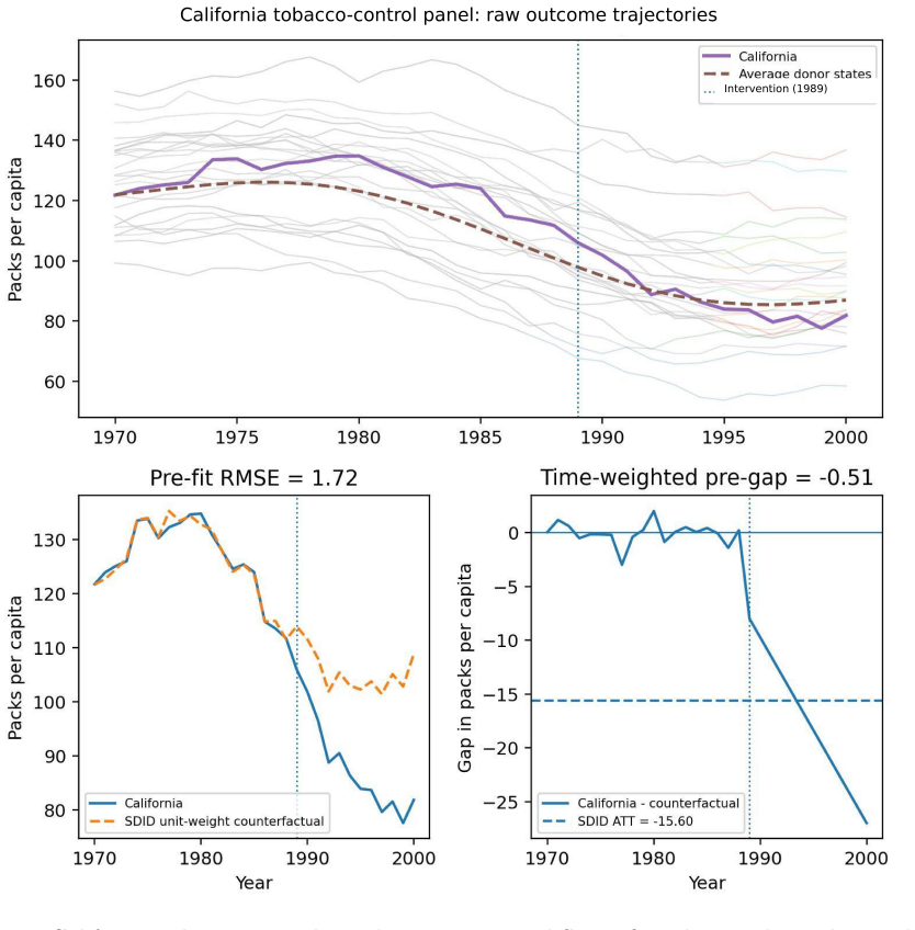
We develop a sensitivity-analysis workflow for causal panel estimators, covering synthetic difference-in-differences, matrix completion, fixed-effect imputation, and group-time average treatment effects. The workflow combines Riesz-representation omitted-variable-bias bounds with partial-$R^2$ robustness values and separates two reporting routes. Route A gives a direct sensitivity profile for additive or projected confounding summarized by outcome-side and Riesz-side partial $R^2$ values. Route B treats observed-covariate benchmarks as auxiliary data only when benchmark-count, alpha-side alignment, model-check, dependence, and dominance diagnostics are credible; otherwise its main role is demotion. We derive estimator-specific Riesz diagnostics and clarify which are fixed-weight, target-level, or first-stage-conditional rather than full derivatives of regularized training maps. Monte Carlo stress tests distinguish calibrated benchmark settings from dominance failure, coarse alpha-side benchmarks, benchmark dependence, noisy covariates, and concentrated SDID weights. In the California tobacco-control panel, the SDID estimate is $-15.60$ packs per capita; corrected finite-donor placebo inference gives standard error 9.49 and add-one $p=0.051$. A refit-weight finite-difference audit changes the Route A nullification robustness value from 0.054 to 0.045, leaving the low-single-digit conclusion unchanged. A county-level minimum-wage application applies the same profile to a multi-cohort staggered panel.
Figures



Reference graph
Works this paper leans on
-
[1]
and Diamond, A
Abadie, A. and Diamond, A. and Hainmueller, J. , year =. Journal of the American Statistical Association , volume =
-
[2]
and Athey, S
Arkhangelsky, D. and Athey, S. and Hirshberg, D. A. and Imbens, G. W. and Wager, S. , year =. American Economic Review , volume =
-
[3]
and Bayati, M
Athey, S. and Bayati, M. and Doudchenko, N. and Imbens, G. and Khosravi, K. , year =. Journal of the American Statistical Association , volume =
-
[4]
, year =
Bai, J. , year =. Econometrica , volume =
-
[5]
and Klaassen, S
Bach, P. and Klaassen, S. and Kueck, J. and Mattes, M. and Spindler, M. , year =
-
[6]
and Feller, A
Ben-Michael, E. and Feller, A. and Rothstein, J. , year =. Journal of the American Statistical Association , volume =
-
[7]
Bissiri, P. G. and Holmes, C. C. and Walker, S. G. , year =. Journal of the Royal Statistical Society Series B: Statistical Methodology , volume =
-
[8]
and Weidner, M
Bonhomme, S. and Weidner, M. , year =. Quantitative Economics , volume =
-
[9]
and Jaravel, X
Borusyak, K. and Jaravel, X. and Spiess, J. , year =. The Review of Economic Studies , volume =
-
[10]
and Sant'Anna, P
Callaway, B. and Sant'Anna, P. H. C. , year =. Journal of Econometrics , volume =
-
[11]
and Chetverikov, D
Chernozhukov, V. and Chetverikov, D. and Demirer, M. and Duflo, E. and Hansen, C. and Newey, W. and Robins, J. , year =. The Econometrics Journal , volume =
-
[12]
and Newey, W
Chernozhukov, V. and Newey, W. and Singh, R. , year =. Econometrica , volume =
-
[13]
and Cinelli, C
Chernozhukov, V. and Cinelli, C. and Newey, W. and Sharma, A. and Syrgkanis, V. , year =. The Review of Economics and Statistics , note =
-
[14]
and Hazlett, C
Cinelli, C. and Hazlett, C. , year =. Journal of the Royal Statistical Society Series B: Statistical Methodology , volume =
-
[15]
and Hazlett, C
Cinelli, C. and Hazlett, C. , year =. Biometrika , volume =
-
[16]
and D'Haultfoeuille, X
de Chaisemartin, C. and D'Haultfoeuille, X. , year =. American Economic Review , volume =
-
[17]
and Masten, M
Diegert, P. and Masten, M. A. and Poirier, A. , year =
-
[18]
and Imbens, G
Doudchenko, N. and Imbens, G. W. , year =
-
[19]
and Pinto, C
Ferman, B. and Pinto, C. , year =. Quantitative Economics , volume =
-
[20]
Frank, K. A. , year =. Sociological Methods & Research , volume =
-
[21]
, year =
Goodman-Bacon, A. , year =. Journal of Econometrics , volume =
-
[22]
and van der Vaart, A
Ghosal, S. and van der Vaart, A. , year =
-
[23]
Grunwald, P. D. and van Ommen, T. , year =. Bayesian Analysis , volume =
-
[24]
Han, S. W. and Mitra, N. and Hettinger, G. and Oganisian, A. , year =
-
[25]
Imbens, G. W. , year =. American Economic Review , volume =
-
[26]
Imbens, G. W. and Wooldridge, J. M. , year =. Journal of Economic Literature , volume =
-
[27]
, year =
Krauth, B. , year =. Journal of Econometric Methods , volume =
-
[28]
Liu, L. and Yamamoto, T. , year =. Political Analysis , volume =. doi:10.1017/pan.2025.10029 , note =
-
[29]
Manski, C. F. , year =. American Economic Review , volume =
-
[30]
Masten, M. A. and Poirier, A. , year =. Econometrica , volume =
-
[31]
Masten, M. A. and Poirier, A. and Zhang, L. , year =. Journal of Business & Economic Statistics , volume =
-
[32]
Miller, J. W. and Dunson, D. B. , year =. Journal of the American Statistical Association , volume =
-
[33]
, year =
Oster, E. , year =. Journal of Business & Economic Statistics , volume =
-
[34]
and Roth, J
Rambachan, A. and Roth, J. , year =. The Review of Economic Studies , volume =
-
[35]
Rosenbaum, P. R. and Rubin, D. B. , year =. Journal of the Royal Statistical Society Series B: Methodological , volume =
-
[36]
and Sant'Anna, P
Roth, J. and Sant'Anna, P. H. C. and Bilinski, A. and Poe, J. , year =. Journal of Econometrics , volume =
-
[37]
Sant'Anna, P. H. C. and Zhao, J. , year =. Journal of Econometrics , volume =
-
[38]
van der Vaart, A. W. , year =
-
[39]
and Hazlett, C
Wainstein, L. and Hazlett, C. , year =
-
[40]
, year =
Xu, Y. , year =. Political Analysis , volume =
-
[41]
VanderWeele, T. J. and Ding, P. , year =. Annals of Internal Medicine , volume =
discussion (0)
Sign in with ORCID, Apple, or X to comment. Anyone can read and Pith papers without signing in.