One Other Option Pricing Scheme

Jimin Lin

One Other Option Pricing Scheme

T0 review · 1 major / 0 minor · reviewed 2026-07-31 · grok-4.5

Challenge this review Re-run · record.json Download PDF Read on arXiv ↗ Review JSON

Pith's one-line read A seven-parameter quantile splice fits a quarter-million SPX volatility curves and yields stable tenor paths.

desk verdict Solid quantile-splice RND with real SPX calibration power and clean math; the arbitrage-free dynamic claim is asserted from visual parameter stability, not shown. read the letter →

arxiv 2607.24680 v1 pith:WYB5EZJ4 submitted 2026-07-27 q-fin.CP math.PR

Jimin Lin This is my paper · ORCID

classification q-fin.CPmath.PR MSC 91G2060E0591G60

keywords optionpricingimpliedvolatilityrisk-neutralquantilesplicestretchedexponentiallocalstaticarbitrageSPXoptions

verification ladder T0 review T1 audit T2 compute T3 formal

The pith

A machine-rendered reading of the paper's core claim, the machinery that carries it, and where it could break.

The reading

Modern short-dated equity options often show implied-volatility curves that are not simply U-shaped: they can be W-shaped, inverse-U, or S-shaped, with local concavity near events. Classical stochastic-volatility or mixture models either need many components or lose interpretability to capture those shapes. This paper parameterizes the risk-neutral quantile function itself by splicing stretched-exponential pieces. A three-segment version with seven free parameters gives direct, localized control over level, wing slope, and central convexity. On two years of SPX and SPXW data the model calibrates essentially every curve to within the bid–ask spread; the fitted parameters form smooth patterns across tenor. Those patterns let one interpolate a whole surface and build a local-volatility dynamics free of static arbitrage. The practical payoff is a single, parsimonious object that both prices today’s book and seeds tomorrow’s process.

What carries the argument

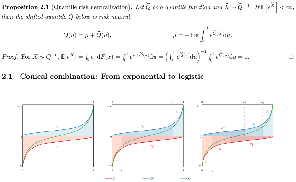
The stretched-exponential quantile splice: the risk-neutral quantile is built piecewise from shifted Weibull quantiles joined C1 at free knots; scale, knot locations and shape exponents give direct, localized control over level, wing slope and central curvature of the implied-volatility curve.

What would settle it

Construct an explicit continuous interpolant of the calibrated seven-parameter paths on a multi-tenor SPX surface, compute the associated Dupire local volatility, and check whether the resulting put prices remain free of calendar-spread arbitrage (partial_tau p >= 0) across a dense grid of tenors and strikes.

Watch

Extended reading notes

Core claim

A risk-neutral stretched-exponential quantile splice with three segments and seven free parameters (global scale, two interior knots, four shape exponents; tails fixed) reproduces the full range of observed SPX implied-volatility shapes—including local concavity—and calibrates accurately to roughly 25 770 curves spanning 2024–2025, with residuals typically inside market spreads and with tenor-stable parameters that support arbitrage-free term-structure interpolation.

Load-bearing premise

That the visually smooth discrete parameter paths across listed tenors can be turned into a continuous term structure that satisfies the integral no-arbitrage condition for every tenor and moneyness.

Editorial extensions

If this is right

A single seven-parameter object prices the bulk of the SPX book to market-spread accuracy.
Stable tenor patterns of the seven parameters allow direct interpolation of entire implied-volatility surfaces.
The same parameter paths seed a Dupire local-volatility diffusion that matches the surface by construction and rules out static arbitrage.
Four-segment or hybrid (affine combination) extensions cover the rare extreme-concavity outliers without leaving the same family.
Wing asymptotics are set a priori by the fixed tail exponents, removing an extra free parameter while still matching observed short-dated wings.

Reading between the lines

Editorial extensions of the paper, not claims the author makes directly.

The same splice construction could be applied day-by-day to single-name or crypto option books where event-driven concavity is even more pronounced.
Because the parameters are directly interpretable, they may serve as low-dimensional state variables for a reduced-form stochastic model of the surface itself.
Hand-tuning the seven parameters without an optimizer already produces usable fits, suggesting the model could be used for rapid scenario generation on a trading desk.

Share X Bluesky LinkedIn Reddit HN

Signed reviews

No signed human review yet.

Editorial analysis

A structured set of objections, weighed in public.

Desk editor's note, referee report, and a circularity audit.

Desk Editor's Note

read the letter

The useful core here is a three-segment stretched-exponential quantile splice (seven free parameters after fixing tails) that gives localized, interpretable control over IV shape, including mild local concavity, and actually fits almost all of 25k SPX/SPXW curves from 2024–25 with residuals inside spreads.

What is new is the specific construction: piecewise Weibull quantiles glued C1, risk-neutralized by the usual additive shift, with explicit wing formulas and a hybrid affine extrapolation for the few extreme W/S shapes. The supporting propositions (risk neutralization, wings, feasible affine combos, local-vol expressions) are standard and carefully written. The empirics are the real strength—hand-crafted intuition, full-day surfaces, residual histograms vs bid–ask, tenor- and moneyness-wise bands, and outlier analysis with four-segment and hybrid fixes. Parameters do show stable tenor patterns (scale grows, knots sit near 0.03/0.98, short-tenor γ1 small). That is genuine engineering value for vol-surface work.

Soft spot, in proportion: the abstract and §6 claim that those patterns “enable term-structure interpolation and dynamic process construction without static arbitrage.” Prop. 6.1 correctly states the integral calendar condition on θ′(τ), but no interpolant is ever built or checked against it. Visual smoothness of the discrete paths is not the same as existence of a feasible direction at every τ (especially short tenors where the γ’s move fastest). Moneyness arbitrage is automatic per slice; calendar is not. So the second headline deliverable is only half-supported. Minor additional limits: closed Bloomberg data, no code, no quantitative baselines against mixtures or SSVI-style params.

This is for people who build or recalibrate equity IV surfaces and want an interpretable RND that handles event-day concavity without jumping to high-component mixtures or nets. Math and residual evidence are solid enough that a serious editor should send it to referees; the dynamic claim just needs an explicit feasible θ(τ) example or a quieter rewrite. I would read the revision and probably cite the splice construction.

Referee Report

1 major / 0 minor

Summary. The paper introduces a family of risk-neutral distributions built by splicing stretched-exponential (Weibull) quantile segments with C¹ matching at knots, closed by an additive risk-neutralizing shift. The three-segment instance has seven free parameters (scale ς, two knots u±₂, four shapes γ±₁, γ±₂) with tail segments fixed. The author develops the construction pedagogically (logistic → beta-logistic → stretched logistic → splice), proves risk-neutralization (Prop. 3.4) and wing asymptotics (Prop. 3.5) from Lee's moment formula and Benaim–Friz, and calibrates independently each of 25,770 SPX/SPXW implied-volatility curves over 2024–2025 (~5M option pairs). Curve-wise RMS implied-vol residuals are reported to lie mostly within RMS half bid–ask spreads; outlier curves with strong concavity are handled by a four-segment model or a hybrid affine combination of two three-segment RNDs, whose feasibility range is characterized (Props. 5.1, 5.4). Section 6 states the calendar no-arbitrage condition (Prop. 6.1) for a parameter term structure θ(τ) and gives Dupire local-volatility formulas (Prop. 6.2, Cor. 6.3).

Significance. The quantile-splice construction is genuinely neat: it exploits the convex-cone structure of quantile functions to obtain a parsimonious, interpretable parameterization with direct, localized control over implied-vol shape, explicit integrability conditions, and closed-form wing asymptotics via Propositions 3.4–3.5 — properties most flexible smile parameterizations lack. The empirical study is large and carefully sliced (curve-, quotation-, tenor-, and moneyness-wise residuals against spreads), and the handcrafted calibration walkthrough (§4.1) substantiates the interpretability claim. The affine-combination feasibility result (Prop. 5.1) and the zero-crossing counting argument (Prop. 5.5, generalizing Glasserman–Pirjol) are clean, correct-looking contributions. If the calibration results hold, this is a practically useful model with an unusually transparent parameter-to-shape mapping, and it would be a solid reference for event-driven concave smiles. The weakest link is the advertised bridge to arbitrage-free surfaces and local-vol dynamics, which is asserted rather than demonstrated.

major comments (1)

The abstract and §6 claim that the stable tenor patterns in the fitted parameters "enable term structure interpolation and dynamic process construction without static arbitrage." This is one of the paper's two headline deliverables, and it is not supported. Proposition 6.1's no-arbitrage condition — for all τ ∈ 𝒯 and all u ∈ (0,1), ∫₀ᵘ e^{Q(v;θ(τ))} ∇_θ Q(v;θ(τ))·θ′(τ) dv ≤ 0 — is a continuum of half-space constraints on the direction θ′(τ) at every tenor, coupling all seven parameter components. Smoothness of the discrete paths {θ̂_t(τ)} in Figs. 5 and 12–14 is neither necessary nor sufficient for feasibility, and no interpolant θ(τ) is ever constructed or checked against the condition. Independent per-component spline interpolation (the natural reading of "interpolation") has no reason to respect it. The short-tenor regime is the sharpest stress point: the initial condition Q(u;θ(0)) =

Circularity Check

0 steps flagged · score 0.0 of 10

No significant circularity: self-contained quantile construction plus empirical calibration; nothing reduces a claimed prediction to its own fitted inputs.

full rationale

This is a model-specification and calibration paper. The stretched-exponential quantile splice is built from explicit operations on Weibull/logistic quantiles (conic combination, composition, monotone transform, C1 piecewise splice) with risk neutralization via the moment condition in Props. 2.1/3.4 and wing formulas from Lee/Benaim–Friz; those steps are definitional constructions, not circular reductions of a target to itself. Empirical success is reported as curve-wise RMS residual versus bid–ask spread after fitting θ to mid prices (Eq. 4.2, Figs. 4–6)—standard calibration evaluation, not a fitted input relabeled as an independent prediction. Props. 5.1–5.5 and 6.1–6.3 derive affine-combination and local-vol consequences of the same construction; they do not redefine the fit. Self-citations (Lin 2026; Lin & Liu 2024) supply background on implied-quantity relations and beta-logistic limitations and are not load-bearing uniqueness or ansatz imports. The Abstract/§6 claim that stable θ̂(τ) patterns “enable” arbitrage-free term-structure interpolation is an under-supported existence assertion (no interpolant is checked against Prop. 6.1), but that is a support gap, not circularity by construction.

Assumptions & free parameters 4 free parameters · 5 assumptions · 2 invented entities

The paper works inside standard risk-neutral pricing. Load-bearing modeling choices are the piecewise stretched-exponential quantile family, fixed tail segments, per-curve free parameters, and the unproven-but-stated integral condition for tenor interpolation. No new physical entities; the invented object is the quantile-splice family itself.

free parameters (4)

Per-curve θ = {ς, u−₂, u+₂, γ−₁, γ−₂, γ+₁, γ+₂} = Example hand fit then optimum on 2024-01-02 τ≈0.1042: {0.06√τ, 0.03, 0.99, 0.33, 0.81, 0.24, 1.22}; full set varies by t
Seven parameters optimized independently for each (t,τ) IV curve under (4.2); central empirical claim depends on these fits.
Fixed tail knots and shapes u−₁=1e-12, u+₁=1-1e-12, γ±₀=1 = Fixed by author choice
Remark 3.2 / §4 choice that presets linear wing asymptotics and reduces parameter count; affects all reported three-segment results.
Segment count M (3 default; 4 or hybrid for outliers) = M=3 for majority; M=4 or λ∈ℝ hybrid for worst concave curves
Model capacity switch used when three-segment residuals are large; hybrid adds λ and a second θ.
Calibration weights w_t(τ,κ) (default squared vega) = Default ν²; vega weight shown as alternative
Changes fits on noisy/challenging curves (§4.4, Fig. 8); not uniquely determined by theory.

assumptions (5)

domain assumption Frictionless risk-neutral pricing: E[e^X]=1; European puts/calls given by (1.1)–(1.2).
Standard Q-measure setup throughout §§1–6.
domain assumption CDFs are continuous and strictly increasing so quantiles exist and are differentiable as used.
Stated in §1.1; required for Q=F^{-1} and q=Q'.
standard math Lee/Benaim–Friz moment and wing formulas (Prop. 1.2) relate tail decay of F to IV wing slopes.
Invoked for Props. 3.5 and earlier logistic/stretched cases.
ad hoc to paper Piecewise Weibull-quantile segments matched C^1 at knots (3.4)–(3.5) define a valid monotone quantile.
Core modeling construction of §3; validity follows from monotone pieces and matching but is a design choice, not a market fact.
standard math A feasible θ(τ) satisfying Prop. 6.1 initial and integral inequalities yields static-arbitrage-free prices and a Dupire local vol.
Classical calendar/vertical/butterfly conditions rewritten in quantile coordinates; existence of such interpolant on market fits is assumed for the dynamic claim.

invented entities (2)

Stretched exponential quantile splice (M-segment risk-neutral model)
purpose: Parsimonious family of RN quantiles with localized control of IV level, wings, and local concavity.
Defined in §3; not a physical particle but a new parametric object on which all empirical claims rest.
Hybrid affine combination of two three-segment splices (F_λ)
purpose: Extrapolate expressivity for extreme W/S-shaped outliers beyond single-splice capacity.
§4.4–§5; λ may lie outside [0,1], so not a mixture—functional extrapolation.

how reviews work

0 comments

Cite this review

Pith. "Pith review of One Other Option Pricing Scheme." pith.science (2026). https://pith.science/paper/WYB5EZJ4

@misc{pith2026260724680,
  author       = {Pith},
  title        = {Pith review of: One Other Option Pricing Scheme},
  year         = {2026},
  howpublished = {\url{https://pith.science/paper/WYB5EZJ4}},
  note         = {Machine review of arXiv:2607.24680}
}

read the original abstract

We present a distinctive approach to parameterizing the risk neutral distribution. Using parsimonious and interpretable parameters, the model provides direct and localized control over the shape of the implied volatility curve. It captures a wide variety of shapes, including those with local concavity. Empirical results demonstrate accurate calibration across a quarter million curves from a two-year Standard and Poor's 500 index option dataset. The fitted parameters exhibit stable patterns across tenors, enabling term structure interpolation and dynamic process construction without static arbitrage.

Figures

Figures reproduced from arXiv: 2607.24680 by the authors.

**Figure 2.** Implied volatility of risk neutral quantiles ( [PITH_FULL_IMAGE:figures/full_fig_p010_2.png] view at source ↗

**Figure 3.** Calibrating a three-segment model to market data on 2024-01-02 with expiration 2024-02-09. [PITH_FULL_IMAGE:figures/full_fig_p015_3.png] view at source ↗

Figures from the paper (11 more)

**Figure 4.** Figure 4: Fitted three-segment model (3.1) for 2024-01-02 over all listed tenors. 17 [PITH_FULL_IMAGE:figures/full_fig_p017_4.png]

**Figure 5.** Figure 5: Fitted parameters (4.4) for 2024-01-02 over all listed tenors. Horizontal axis is tenor. wing becomes flatter for longer tenors. The shape parameter for the major intervals, 𝛾 ± 2 , on the other hand, is large at short tenors and evolves differently as tenor increases,…

**Figure 6.** Figure 6: Root mean square residuals (red) versus root mean square spread (green). Top left: curve-wise ( [PITH_FULL_IMAGE:figures/full_fig_p019_6.png]

**Figure 7.** Figure 7: Refining worst fits. Each column presents fits by three models to the same data. First row: three [PITH_FULL_IMAGE:figures/full_fig_p021_7.png]

**Figure 8.** Figure 8: Alternative fits with more noticeable bimodality in implied density. [PITH_FULL_IMAGE:figures/full_fig_p023_8.png]

**Figure 9.** Figure 9: Calibration for 2024-06-03. 31 [PITH_FULL_IMAGE:figures/full_fig_p031_9.png]

**Figure 10.** Figure 10: Calibration for 2025-01-02. 32 [PITH_FULL_IMAGE:figures/full_fig_p032_10.png]

**Figure 11.** Figure 11: Calibration for 2025-04-30. 33 [PITH_FULL_IMAGE:figures/full_fig_p033_11.png]

**Figure 12.** Figure 12: Fitted parameters for 2024-06-03. 0.0 0.5 1.0 1.5 0.00 0.02 0.04 0.06 0.08 0.10 0.0 0.5 1.0 1.5 0.0 0.2 0.4 0.6 0.8 1.0 0.0 0.5 1.0 1.5 0.0 0.6 1.2 1.8 2.4 3.0 0.0 0.5 1.0 1.5 0.0 0.6 1.2 1.8 2.4 3.0 [PITH_FULL_IMAGE:figures/full_fig_p034_12.png]

**Figure 13.** Figure 13: Fitted parameters for 2025-01-02. 0.0 0.4 0.8 1.2 0.00 0.03 0.06 0.09 0.12 0.15 0.0 0.4 0.8 1.2 0.0 0.2 0.4 0.6 0.8 1.0 0.0 0.4 0.8 1.2 0.0 0.6 1.2 1.8 2.4 3.0 0.0 0.4 0.8 1.2 0.0 0.6 1.2 1.8 2.4 3.0 [PITH_FULL_IMAGE:figures/full_fig_p034_13.png]

**Figure 14.** Figure 14: Fitted parameters for 2025-04-30. 34 [PITH_FULL_IMAGE:figures/full_fig_p034_14.png]

Discussion (0). Continue with ORCID to comment.

Reference graph

Works this paper leans on

29 extracted references · 2 linked inside Pith

[1]

Tagasovska, and T

Ackerer, D., N. Tagasovska, and T. Vatter (2020). Deep smoothing of the implied volatility surface. Advances in Neural Information Processing Systems 33 , 11552–11563. 28

2020
[2]

Goyal, A

Alexiou, L., A. Goyal, A. Kostakis, and L. Rompolis (2025). Pricing event risk: Evidence from concave implied volatility curves. Review of Finance 29 (4), 963–1007

2025
[3]

Azzone, M. and L. Torricelli (2025). Explicit option pricing with additive processes. SIAM Journal on Financial Mathematics 16 (3), 747–802

2025
[4]

Gillberg, and S

Baker, M., T. Gillberg, and S. Thomas (2018). Trading events: Smiles, frowns and moustaches–the many faces of the options market. SSRN 3263368

2018
[5]

Benaim, S. and P. Friz (2009). Regular variation and smile asymptotics. Mathematical Finance 19 (1), 1–12

2009
[6]

Brigo, D. and F. Mercurio (2002). Lognormal-mixture dynamics and calibration to market volatility smiles. International Journal of Theoretical and Applied Finance 5 (04), 427–446

2002
[7]

Brunner, B. and R. Hafner (2003). Arbitrage-free estimation of the risk-neutral density from the implied volatility smile. Journal of Computational Finance 7 (1), 75–106

2003
[8]

Carr, P. and L. Torricelli (2021). Additive logistic processes in option pricing. Finance and Stochas- tics 25 (4), 689–724

2021

Show all 29 references

[9]

Dupire, B. (1994). Pricing with a smile. Risk 7 (1), 18–20

1994
[10]

Durrleman, V. (2010). Implied volatility: Market models. Encyclopedia of Quantitative Finance

2010
[11]

Gilchrist, W. (2000). Statistical modelling with quantile functions . Chapman and Hall/CRC

2000
[12]

Glasserman, P. and D. Pirjol (2023). W-shaped implied volatility curves and the Gaussian mixture model. Quantitative Finance 23 (4), 557–577

2023
[13]

Homescu, C. (2011). Implied volatility surface: Construction methodologies and characteristics. arXiv 1107.1834

2011 arXiv
[14]

Itkin, A. (2015). To sigmoid-based functional description of the volatility smile. The North American Journal of Economics and Finance 31 , 264–291

2015
[15]

Jackwerth, J. C. (2000). Recovering risk aversion from option prices and realized returns. The Review of Financial Studies 13 (2), 433–451

2000
[16]

Keelin, T. W. (2016). The metalog distributions. Decision Analysis 13 (4), 243–277

2016
[17]

Keller-Ressel, M. (2025). W-shaped implied volatility curves in a variance-gamma mixture model. Frontiers of Mathematical Finance 6 , 1–15

2025
[18]

Keller-Ressel, M. and H. Nikulski (2026). Discovering parametrizations of implied volatility with sym- bolic regression. arXiv 2603.21892 . 29

2026
[19]

Klassen, T. (2023). State of the smile: The ever-surprising evolution of the equity/listed options market. VolaDynamics

2023
[20]

Lee, R. W. (2004). The moment formula for implied volatility at extreme strikes. Mathematical Fi- nance 14(3), 469–480

2004
[21]

Lin, J. (2026). Shallow representation of option implied information. arXiv 2603.17151

2026
[22]

Lin, J. and G. Liu (2024). Neural term structure of additive process for option pricing. In Proceedings of the 5th ACM International Conference on AI in Finance , pp. 695–702

2024
[23]

Roper, M. (2009). Implied volatility: General properties and asymptotics . Ph. D. thesis, UNSW Sydney

2009
[24]

Tavin, B. (2012). Implied distribution as a function of the volatility smile. Bankers Markets and Investors (119), 31–42

2012
[25]

Jacquier, and L

Wiedemann, R., A. Jacquier, and L. Gonon (2024). Operator deep smoothing for implied volatility. arXiv 2406.11520

2024 arXiv
[26]

Yang, Y., W. Chen, C. Shu, and T. Hospedales (2025). Hyperiv: Real-time implied volatility smoothing. In The 42nd International Conference on Machine Learning , pp. 1–15. PMLR

2025
[27]

Zaugg, N. F., L. Perotti, and L. A. Grzelak (2025). Volatility parametrizations with random coeﬀicients: Analytic flexibility for implied volatility surfaces. SIAM Journal on Financial Mathematics 16 (4), 1374– 1411

2025
[28]

Yang, and B

Zheng, Y., Y. Yang, and B. Chen (2021). Incorporating prior financial domain knowledge into neural networks for implied volatility surface prediction. In Proceedings of the 27th ACM SIGKDD Conference on Knowledge Discovery & Data Mining , pp. 3968–3975

2021
[29]

Zhou, S. (2025). 0dte smile dynamics and jump diffusion models. Lecture slides, NYU Tandon. A Additional results 30 −0.02 0.000.0 0.2 0.4 0.6 0.8 1.0 −0.05 0.00 −0.10 −0.05 0.00 −0.10 0.00 −0.20 −0.10 0.00 −0.20 −0.10 0.00 −0.20 0.000.0 0.2 0.4 0.6 0.8 1.0 −0.20 0.00 −0.20 0.0...

2025

Pith tools

Reviewed July 31, 2026 · model on record in the stance chip above.

[1] [1]

Tagasovska, and T

Ackerer, D., N. Tagasovska, and T. Vatter (2020). Deep smoothing of the implied volatility surface. Advances in Neural Information Processing Systems 33 , 11552–11563. 28

2020

[2] [2]

Goyal, A

Alexiou, L., A. Goyal, A. Kostakis, and L. Rompolis (2025). Pricing event risk: Evidence from concave implied volatility curves. Review of Finance 29 (4), 963–1007

2025

[3] [3]

Azzone, M. and L. Torricelli (2025). Explicit option pricing with additive processes. SIAM Journal on Financial Mathematics 16 (3), 747–802

2025

[4] [4]

Gillberg, and S

Baker, M., T. Gillberg, and S. Thomas (2018). Trading events: Smiles, frowns and moustaches–the many faces of the options market. SSRN 3263368

2018

[5] [5]

Benaim, S. and P. Friz (2009). Regular variation and smile asymptotics. Mathematical Finance 19 (1), 1–12

2009

[6] [6]

Brigo, D. and F. Mercurio (2002). Lognormal-mixture dynamics and calibration to market volatility smiles. International Journal of Theoretical and Applied Finance 5 (04), 427–446

2002

[7] [7]

Brunner, B. and R. Hafner (2003). Arbitrage-free estimation of the risk-neutral density from the implied volatility smile. Journal of Computational Finance 7 (1), 75–106

2003

[8] [8]

Carr, P. and L. Torricelli (2021). Additive logistic processes in option pricing. Finance and Stochas- tics 25 (4), 689–724

2021