REVIEW 2 major objections 5 minor 35 references
Nonnegative Low-Rank Matrix Correction under an Orthogonality Constraint in Conservative Vlasov Simulations
T0 review · 2 major / 5 minor · reviewed 2026-08-01 · deepseek-v4-flash
Pith's one-line read Nonnegative low-rank corrections to Vlasov solutions reduce to an implicit singular-value thresholding rule, enabling five convex algorithms and a tangent-space method that preserve mass, momentum, and energy.
desk verdict A genuine new proximal characterization and a fast tangent-space projection algorithm, undercut by a false feasibility condition and under-specified dual gradient steps. read the letter →
The pith
A machine-rendered reading of the paper's core claim, the machinery that carries it, and where it could break.
The reading
What carries the argument
The central object is the proximal operator of g(Y)=||Y||_*^2+(a2/2)||Y||_F^2+I_{YB=0}; Theorem 1 characterizes it as implicit singular value soft-thresholding with threshold τ=2||Y||_*/(a2+η), computed from the root of 0=(a2+η)τ−2Σ_k max{σ_k−τ,0}. This single identity carries the convex algorithms (Douglas–Rachford splitting, restarted dual FISTA, accelerated gradient, PR+ conjugate gradient, L-BFGS). For the non-convex formulation, the carrying mechanism is the tangent-space projection P_{T_{M_{r,B}}(X)}(Y)=P_{T_{M_r}(X)}(YΠ^⊥_B), which reduces each alternating-projection step to a 2r×2r SVD while keeping the iterate in rank-r factored form and satisfying XB=0 exactly.
What would settle it
Compute the proximal operator for a small random instance (e.g., 2×3 with a chosen orthonormal B) by brute-force convex optimization and compare with the implicit threshold formula (25); a mismatch anywhere in the threshold bisection would refute Theorem 1. Separately, take moments with ρ>0 and eρ<m² and confirm the algorithms cannot return a nonnegative A+X, which would confirm the infeasibility boundary stated in Remark 2.
Extended reading notes
Core claim
The central discovery is Theorem 1: for the correction problem min_X ||X||_*^2 + (a/2)||X||_F^2 subject to X≥−A and XB=0, the proximal operator of the orthogonality-constrained squared nuclear norm has the closed-form characterization Y = D_{2||Y||_*/(a2+η)}(η/(a2+η) M Π^⊥_B), an implicit equation because the threshold depends on the nuclear norm of the unknown minimizer. The paper shows the threshold is the unique root of a convex piecewise-linear scalar equation, computable by bisection after one SVD of MΠ^⊥_B. This makes the convex problem globally solvable by any of five proposed algorithms and makes the non-convex rank-constrained formulation solvable by tangent-space accelerated altern
Load-bearing premise
The admissible set must be nonempty: there has to exist a nonnegative matrix with the same first three velocity moments as the input; the paper gives the condition ρ>0 and eρ≥m² (Remark 2), and if it fails, no correction exists and every algorithm and the central claim collapse.
Editorial extensions
If this is right
- A positivity limiter based on this correction can be embedded in a conservative low-rank Vlasov solver; it removes truncation-induced negative entries while conserving mass, momentum, and energy pointwise.
- Because all five convex algorithms provably reach the same global minimizer, the correction quality does not depend on which solver is chosen, only on the penalty parameter a.
- The tangent-space accelerated alternating projection keeps XB=0 exactly at every iterate, so when used as a limiter it preserves the three conserved moments to machine precision, whereas the Douglas–Rachford limiter preserves them only to its convergence tolerance.
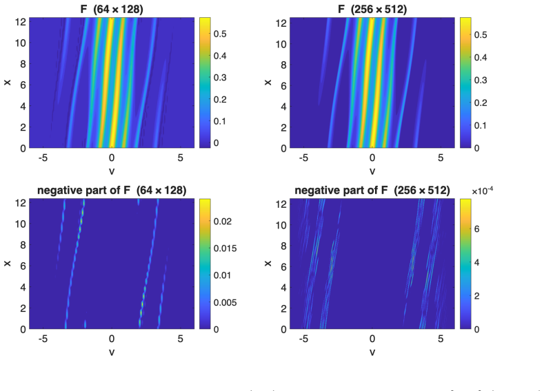
- Residual negativity after storage is set by the re-truncation tolerance of the low-rank format, not by the correction itself; tightening the tolerance drives negativity toward machine precision at a modest, sub-linear rank increase.
- The per-iteration cost gap between the convex methods (full m×n SVD) and TAP (2r×2r SVD) grows with problem size, so TAP becomes increasingly cost-competitive as grids refine.
Reading between the lines
- The implicit-threshold proximal operator is a generic primitive: any optimization with a squared nuclear norm objective and a linear constraint XB=0 (e.g., matrix denoising with a known column subspace) could reuse this bisection-based solver.
- The feasibility condition ρ>0 and eρ≥m², if violated, means no nonnegative distribution can have those first three moments; then the correction problem is infeasible and the solver would need to adjust the moments themselves, not just the matrix entries.
- The TAP idea of projecting onto the tangent space of the rank-and-orthogonality manifold before truncation likely extends to tensor-train or other low-rank formats, where a full SVD is prohibitively expensive.
- Because the correction is operator-agnostic, the same limiter should apply to Fokker–Planck or other kinetic equations where nonnegativity is required, not just Vlasov–Poisson.
Signed reviews
Editorial analysis
A structured set of objections, weighed in public.
Referee Report
Summary. The paper proposes optimization-based post-processing to restore nonnegativity in low-rank Vlasov simulations while preserving the macroscopic moments (density, momentum, and energy). The correction X must satisfy A+X ≥ 0 and XB = 0, where B encodes the discrete moment basis. The central theoretical result (Theorem 1) characterizes the proximal operator of the squared nuclear norm subject to the orthogonality constraint XB = 0 as an implicit singular-value soft-thresholding map, with the threshold determined by a scalar root-finding problem. On this basis the authors develop Douglas–Rachford splitting and four dual first-order methods for the convex formulation (2), and a tangent-space accelerated alternating projection (TAP) for the rank-constrained nonconvex formulation (17). Numerical experiments on Landau damping and a bump-on-tail LoMaC low-rank run compare the algorithms, measure per-iteration cost scaling, and demonstrate the correction as a positivity limiter inside a time-dependent conservative solver.
Significance. If the proximal characterization in Theorem 1 is correct, it is a useful addition to the toolkit for spectral-norm regularization with linear constraints; the bisection threshold makes the proximal operator implementable. The TAP algorithm is attractive because it avoids full SVDs, keeps the orthogonality constraint exact at every iterate, and the numerical scaling study is informative. The paper also includes worthwhile fairness checks: a naive baseline, a randomized-SVD comparison, and tuned step sizes in the cost-scaling study. The main caveats are the incorrect discrete feasibility condition in Remark 2 and under-specified gradient evaluations for the dual algorithms; both affect the validity or reproducibility of the claims as currently stated.
major comments (2)
- [§3.2, Remark 2] The claimed necessary and sufficient condition for non-emptiness of the admissible set is false on a discrete grid. For v ∈ {−1,0,1}, take one row of A to be [1,−1,1]. Then (ρ,m,e) = (1,0,2), so ρ > 0 and eρ ≥ m², yet no nonnegative vector y on this grid can have these moments: e = Σ v_j² y_j ≤ Σ y_j = ρ, while here e = 2 > ρ = 1. The finite-grid moment cone is strictly smaller than the continuous Hamburger cone. Since an empty admissible set makes every proposed correction algorithm meaningless, the paper should either state the correct discrete moment-cone condition or verify feasibility for the test data and restrict the existence claim to the continuous setting.
- [§4.3–§4.4, Eq. (42)] The gradient ∇g*(Λ) is used by dual FISTA variant II, dual accelerated gradient descent, PR+ conjugate gradient, and L-BFGS, but Eq. (42) defines X only implicitly: X = D_{2||X||_*/a2}(a2^{-1}ΛΠ_B^⊥). The manuscript never states that evaluating this map requires solving the scalar threshold equation a2 τ = 2 Σ max(σ_i−τ,0) by bisection, nor does it derive (42). As written, these four algorithms are not fully specified. Please add the derivation and the root-finding step, or explicitly reduce to the a2=0/η=a2 case of Theorem 1.
minor comments (5)
- [§4.2, Remark 3] The function h(τ) = (a2+η)τ − 2Σ max(σ_k−τ,0) is strictly increasing and piecewise linear, but it is concave, not convex: its derivative (a2+η) + 2·#{σ_k > τ} decreases as τ increases. Monotonicity is enough for the bisection argument; please correct the wording.
- [§4.2, Theorem 1 proof] The proof says it constructs a candidate via (25), but (25) is implicit and the threshold root (31) is only introduced in Remark 3 after the theorem. Reorganizing the proof as: define τ as the unique root of (31), set Y = D_τ(η/(a2+η) M Π_B^⊥), and then verify the optimality conditions, would remove the appearance of circularity and shorten the argument.
- [§3.2, Eqs. (33)–(34)] The conjugate formulas (33)–(34) are stated with almost no derivation. In particular, (34) relies on a spectral conjugate calculation that is not evident from the text. A short derivation or a reference to the spectral-conjugate calculus would improve reproducibility.
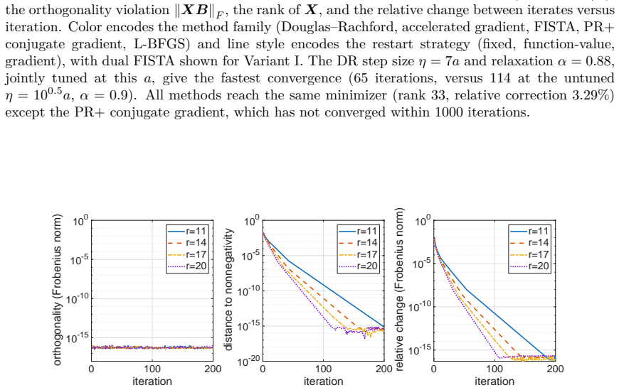
- [§4.3 and Table 1] The text says all convex algorithms converge to the same global minimizer, but Table 1 reports that PR+ conjugate gradient does not meet the tolerance within 1000 iterations and has not reached rank 33. Please qualify the statement to refer to the converged runs.
- [Data availability] The paper states that data and code are available from the authors upon request. For a numerical paper with a cost-scaling comparison, a persistent repository link would substantially aid reproducibility.
Circularity Check
No significant circularity: Theorem 1 is derived in-text from KKT/subgradient conditions, algorithm outputs are measured against an algebraic lower bound, and the paper's self-citations are provenance/setup rather than load-bearing.
full rationale
The derivation chain is self-contained at its load-bearing point. Theorem 1 (Sec. 4.2.2) characterizes the proximal operator of the orthogonality-constrained squared nuclear norm as an implicit singular value thresholding map; the proof starts from the KKT system (23)-(27), uses Lemma 1 (proved in-text) and the standard subdifferential of the nuclear norm (Prop. 1), and verifies that a candidate built from the self-consistency equation (31) satisfies optimality. The proximal problem (22) (input) and the implicit SVT characterization (25) (output) are not equivalent by construction: the subgradient verification is genuine content, and the bisection in Remark 3 is a root-finding procedure on that derived fixed-point condition, not a fitted parameter. Formulation (2) is justified in-text by consistency and homogeneity (Example 1), so it is not a renamed known result. All five convex algorithms and TAP are standard optimization methods applied to (2)/(17); the reported corrections (3.29%/3.31% versus the algebraic lower bound 3.08% = ||min{A,0}||_F/||A||_F), conserved-moment deviations (~1e-14), and per-iteration cost scalings (Tables 2-3, Fig. 6) are measured, not fitted, and hyperparameters (a=1000, eta=7a, alpha=0.88) are explicitly reported as tuned. Self-citations ([13],[14] by Guo/Qiu for the LoMaC setup and solver; [35] by Zheng/Vandereycken/Zhang for standard fixed-rank tangent-space facts) are not load-bearing: the moment-preservation equivalence XB=0 <-> X sqrt(S) R^T = 0 is derived algebraically in Secs. 2.2-2.3, and conservation is independently measured in Table 5. The reviewer-flagged feasibility condition of Remark 2 (rho>0 and e*rho>=m^2 as necessary and sufficient) is a potential correctness gap on discrete velocity grids, not a circularity, since no output is derived from it and test-data feasibility is evidenced by the computed min(A+X)=0. The paper also states its own limitations honestly (DR enforces XB=0 only in the limit; fixed rank caps attainable nonnegativity; limited-solution rank grows sub-linearly, Sec. 5.5 and Fig. 8), which corroborates rather than undermines the non-circularity verdict.
Assumptions & free parameters
free parameters (5)
- Penalty parameter a =
1000
- DR splitting parameters a1, a2 =
a/2 each
- DR step size η and relaxation α =
η=7a, α=0.88
- TAP rank r =
20 (fixed test), N+3 (limiter)
- Re-truncation tolerance εtr =
1e-4 or 1e-10
assumptions (6)
- domain assumption F = F1 + F2 with F1 rank-3 carrying the macroscopic moments and F2 having zero velocity moments (F2 R^T = 0)
- domain assumption Rescaling by the positive diagonal matrix S maps the weighted velocity-space inner product to the Frobenius inner product
- domain assumption Feasibility of the admissible set: there exists a nonnegative matrix with the same first three velocity moments; iff ρ>0 and e·ρ ≥ m²
- standard math Subdifferential of the nuclear norm (Proposition 1) and Moreau decomposition
- standard math Tangent-space characterization and least-squares projection formulas for fixed-rank manifolds from [29,35]
- domain assumption The low-rank solution remains genuinely low rank after correction and re-truncation
Cite this review
Pith. "Pith review of Nonnegative Low-Rank Matrix Correction under an Orthogonality Constraint in Conservative Vlasov Simulations." pith.science (2026). https://pith.science/paper/7SHKNGQK
@misc{pith2026260726272,
  author       = {Pith},
  title        = {Pith review of: Nonnegative Low-Rank Matrix Correction under an Orthogonality Constraint in Conservative Vlasov Simulations},
  year         = {2026},
  howpublished = {\url{https://pith.science/paper/7SHKNGQK}},
  note         = {Machine review of arXiv:2607.26272}
}
abstract
In low-rank numerical methods for Vlasov dynamics, the SVD-type truncation procedure may introduce negative entries into the numerical solution. Such negative values are unphysical because the solution is a probability distribution function. We design optimization-based post-processing algorithms to recover nonnegativity while preserving the macroscopic quantities (density, momentum, and energy) pointwise. The preservation of the macroscopic quantities is written as an orthogonality constraint on the correction term. For a convex formulation based on squared nuclear norm minimization, we show that the proximal operator with the orthogonality constraint is characterized by an implicit singular value thresholding equation, and the threshold can be computed efficiently by bisection. Based on this result, we develop five algorithms for the convex formulation: Douglas--Rachford splitting, restarted dual FISTA, restarted dual accelerated gradient descent, dual PR+ conjugate gradient, and dual L-BFGS. We also consider a non-convex formulation with an explicit rank constraint and develop a tangent-space accelerated alternating projection algorithm that only requires a \(2r \times 2r\) SVD per iteration. Numerical results for a Landau damping test case show that the proposed algorithms give comparable correction quality. Among them, the tangent-space accelerated alternating projection is the most cost-efficient, increasingly so as the problem size grows. We further demonstrate the correction as a positivity limiter inside a time-dependent conservative low-rank Vlasov solver, where it removes the negativity introduced by the SVD-type truncation while preserving the conserved mass, momentum, and energy.
Figures


Figures from the paper (5 more)


Reference graph
Works this paper leans on
-
[1]
A. Beck. First-Order Methods in Optimization , volume 25 of MOS-SIAM Series on Optimiza- tion. SIAM, Philadelphia, PA, 2017
2017
-
[2]
Beck and M
A. Beck and M. Teboulle. A fast iterative shrinkage-thresholding algorithm for linear inverse problems. SIAM Journal on Imaging Sciences , 2(1):183–202, 2009
2009
-
[3]
J.-F. Cai, E. J. Candès, and Z. Shen. A singular value thresholding algorithm for matrix completion. SIAM Journal on optimization , 20(4):1956–1982, 2010
1956
-
[4]
Ceruti, J
G. Ceruti, J. Kusch, and C. Lubich. A rank-adaptive robust integrator for dynamical low-rank approximation. BIT Numerical Mathematics , 62(4):1149–1174, 2022
2022
-
[5]
Ceruti and C
G. Ceruti and C. Lubich. An unconventional robust integrator for dynamical low-rank approx- imation. BIT Numerical Mathematics , 62(1):23–44, 2022
2022
-
[6]
Y. Chen, D. Xiu, and X. Zhang. On enforcing non-negativity in polynomial approximations in high dimensions. SIAM Journal on Scientific Computing , 47(2):A866–A888, 2025
2025
-
[7]
Dektor and L
A. Dektor and L. Einkemmer. Interpolatory dynamical low-rank approximation for the 3+ 3d Boltzmann-BGK equation. Journal of Computational Physics , 547:114515, 2026
2026
-
[8]
Einkemmer and I
L. Einkemmer and I. Joseph. A mass, momentum, and energy conservative dynamical low-rank scheme for the Vlasov equation. Journal of Computational Physics , 443:110495, 2021. 36
2021
Show all 35 references
-
[9]
Einkemmer, K
L. Einkemmer, K. Kormann, J. Kusch, R. G. McClarren, and J.-M. Qiu. A review of low- rank methods for time-dependent kinetic simulations. Journal of Computational Physics , 538:114191, 2025
2025
-
[10]
S. A. Goreinov, I. V. Oseledets, D. V. Savostyanov, E. E. Tyrtyshnikov, and N. L. Zamarashkin. How to find a good submatrix. In V. Olshevsky and E. Tyrtyshnikov, editors, Matrix Methods: Theory, Algorithms and Applications , pages 247–256. World Scientific, 2010
2010
-
[11]
W. Guo, J. F. Ema, and J.-M. Qiu. A local macroscopic conservative (lomac) low rank tensor method with the discontinuous Galerkin method for the Vlasov dynamics. Communications on Applied Mathematics and Computation , 6(1):550–575, 2024
2024
-
[12]
Guo and J.-M
W. Guo and J.-M. Qiu. A low rank tensor representation of linear transport and nonlinear Vlasov solutions and their associated flow maps. Journal of Computational Physics , 458:111089, 2022
2022
-
[13]
Guo and J.-M
W. Guo and J.-M. Qiu. A conservative low rank tensor method for the Vlasov dynamics. SIAM Journal on Scientific Computing , 46(1):A232–A263, 2024
2024
-
[14]
Guo and J.-M
W. Guo and J.-M. Qiu. A local macroscopic conservative (LoMaC) low rank tensor method for the Vlasov dynamics. Journal of Scientific Computing , 101(3):61, 2024
2024
-
[15]
Halko, P.-G
N. Halko, P.-G. Martinsson, and J. A. Tropp. Finding structure with randomness: probabilistic algorithms for constructing approximate matrix decompositions. SIAM Review, 53(2):217–288, 2011
2011
-
[16]
Koch and C
O. Koch and C. Lubich. Dynamical low-rank approximation. SIAM Journal on Matrix Analysis and Applications, 29(2):434–454, 2007
2007
-
[17]
Lions and B
P.-L. Lions and B. Mercier. Splitting algorithms for the sum of two nonlinear operators. SIAM Journal on Numerical Analysis , 16(6):964–979, 1979
1979
-
[18]
C. Liu, D. Milesis, C.-W. Shu, and X. Zhang. Efficient optimization-based invariant-domain- preserving limiters in solving gas dynamics equations. Journal of Computational Physics , 558:114839, 2026
2026
-
[19]
D. C. Liu and J. Nocedal. On the limited memory BFGS method for large scale optimization. Mathematical Programming, 45(1–3):503–528, 1989
1989
-
[20]
Lubich and I
C. Lubich and I. V. Oseledets. A projector-splitting integrator for dynamical low-rank approx- imation. BIT Numerical Mathematics , 54(1):171–188, 2014
2014
-
[21]
Y. E. Nesterov. A method of solving a convex programming problem with convergence rate o( 1 k2 ). Doklady Akademii Nauk SSSR , 269(3):543–547, 1983
1983
-
[22]
Y. E. Nesterov. Gradient methods for minimizing composite functions. Mathematical Pro- gramming, 140(1):125–161, Aug 2013
2013
-
[23]
O’Donoghue and E
B. O’Donoghue and E. J. Candès. Adaptive restart for accelerated gradient schemes. Founda- tions of Computational Mathematics , 15(3):715–732, Jun 2015. 37
2015
-
[24]
Perthame and C.-W
B. Perthame and C.-W. Shu. On positivity preserving finite volume schemes for Euler equa- tions. Numerische Mathematik , 73(1):119–130, 1996
1996
-
[25]
M. J. D. Powell. Convergence properties of algorithms for nonlinear optimization. SIAM Review, 28(4):487–500, 1986
1986
-
[26]
G.-J. Song, M. K. Ng, and T.-X. Jiang. Tangent space based alternating projections for nonnegative low rank matrix approximation. IEEE Transactions on Knowledge and Data Engineering, 35(11):11917–11934, 2023
2023
-
[27]
Sun and J
J. Sun and J. Zhang. Global convergence of conjugate gradient methods without line search. Annals of Operations Research , 103(1–4):161–173, Mar 2001
2001
-
[28]
X. Tang, R. Dwaraknath, and L. Ying. Variational inference and density estimation with non-negative tensor train. arXiv preprint arXiv:2507.21519 , 2025
2025 arXiv
-
[29]
Vandereycken
B. Vandereycken. Low-rank matrix completion by Riemannian optimization. SIAM Journal on Optimization , 23(2):1214–1236, 2013
2013
-
[30]
K. Wu, X. Zhang, and C.-W. Shu. High order numerical methods preserving invariant domain for hyperbolic and related systems. arXiv preprint arXiv:2512.09116 , 2025
2025
-
[31]
Ye and N
E. Ye and N. F. G. Loureiro. Quantized tensor networks for solving the Vlasov–Maxwell equations. Journal of Plasma Physics , 90(3):805900301, 2024
2024
-
[32]
Zhang and C.-W
X. Zhang and C.-W. Shu. On positivity-preserving high order discontinuous Galerkin schemes for compressible Euler equations on rectangular meshes. Journal of Computational Physics , 229(23):8918–8934, 2010
2010
-
[33]
Zheng, D
N. Zheng, D. Hayes, A. Christlieb, and J.-M. Qiu. A Semi-Lagrangian adaptive-rank (SLAR) method for linear advection and nonlinear Vlasov-Poisson system. Journal of Computational Physics, 532:113970, 2025
2025
-
[34]
Zheng, W
N. Zheng, W. A. Sands, D. Hayes, A. J. Christlieb, and J.-M. Qiu. A semi-Lagrangian adaptive rank (SLAR) method for high-dimensional Vlasov dynamics. SIAM Journal on Scientific Computing, page accepted, 2026
2026
-
[35]
Zheng, W
S. Zheng, W. Huang, B. Vandereycken, and X. Zhang. Riemannian optimization using three different metrics for Hermitian PSD fixed-rank constraints. Computational Optimization and Applications, 91(3):1135–1184, 2025. 38
2025
Reviewed August 1, 2026 · model on record in the stance chip above.
Discussion (0). Continue with ORCID to comment.