Random punctured hyperbolic surfaces & the Brownian sphere

Nicolas Curien; Timothy Budd

REVIEW 3 major objections 3 minor 1 cited by

Random punctured hyperbolic surfaces & the Brownian sphere

T0 review · 3 major / 3 minor · reviewed 2026-08-05 · deepseek-v4-flash

Challenge this review Re-run · record.json Download PDF Read on arXiv ↗

Pith's one-line read Random Weil-Petersson spheres with many cusps converge to the Brownian sphere after n^{-1/4} rescaling.

desk verdict Major advance: WP punctured spheres join the Brownian sphere universality class via a new Schaeffer-type tree encoding, but the ε→0 step in Theorem 3 and two smaller gaps need attention before I'd call it watertight. read the letter →

arxiv 2508.18792 v1 pith:3ASPC7UT submitted 2025-08-26 math.PR math-phmath.GTmath.MP

Timothy Budd , Nicolas Curien This is my paper · ORCID

classification math.PRmath-phmath.GTmath.MP MSC 60D0560F1732G15

keywords randomhyperbolicsurfacesWeil-PeterssonmeasureBrownianspherelabeledtreeencodingBenjamini-SchrammconvergenceGromov-Hausdorff-Prokhorovplanarmapspuncturedspheres

verification ladder T0 review T1 audit T2 compute T3 formal

The pith

A machine-rendered reading of the paper's core claim, the machinery that carries it, and where it could break.

The reading

The paper asks what a typical large hyperbolic sphere with many punctures looks like when sampled from the natural Weil-Petersson measure, and answers with a precise two-scale description. Globally, after cutting off unit horocycle collars around the punctures and rescaling the hyperbolic metric by $n^{-1/4}$, the random surface converges in distribution to the Brownian sphere, with an explicit constant $c_{wp} = 2\pi \sqrt{3}/c_0 \approx 2.3392$; the same holds for the measured surface carrying normalized hyperbolic area. Locally, without rescaling, a typical point sees an infinite hyperbolic surface homeomorphic to $\mathbb{R}^2 \setminus \mathbb{Z}^2$ with countably many cusps. To get there, the paper builds a tree encoding of a punctured sphere by a plane binary tree whose corners carry angles, and proves that the Weil-Petersson measure becomes Lebesgue measure on allowed angle configurations. That reduction moves the problem into the well-developed realm of random labeled trees and their scaling limits.

What carries the argument

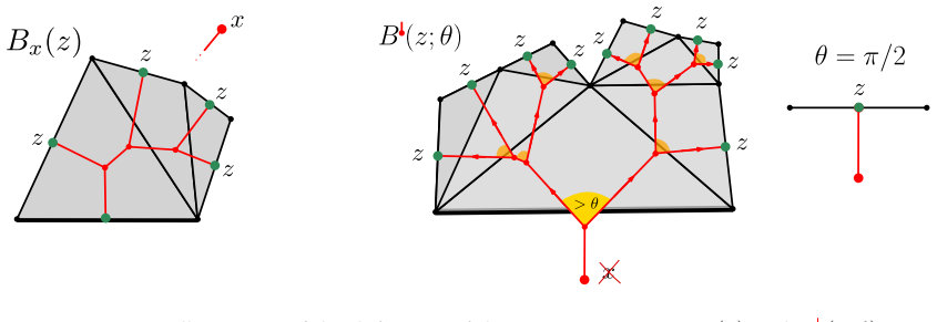
The key object is the allowed-angle binary tree encoding of a punctured sphere. Starting from $\lambda$-length coordinates on decorated ideal triangles, the paper lets every horocycle except the origin's shrink to a point; the cut-locus of the origin becomes a plane binary tree whose leaves are the other punctures, and the Euclidean triangles built from $\lambda$-lengths place angles in $(0,\pi)$ at each corner. The global constraint that opposite angles around each internal edge sum to more than $\pi$ is exactly the Delaunay condition. Theorem 3 shows the Weil-Petersson measure is $2^{n-2}$ times Lebesgue measure on such configurations. The analytic work then decomposes the associated tree of Euclidean tri

What would settle it

Take a small fixed $n$, enumerate the finitely many rooted plane binary trees with $n$ leaves, integrate Lebesgue measure over each allowed-angle polytope, and compare the total with Zograf's exact Weil-Petersson volume through the paper's formula relating the two; a mismatch beyond numerical precision would refute Theorem 3 and with it the whole route. For the scaling limit itself, simulate the $n$-horocycle distance matrix for a large $n$, rescale by $n^{-1/4}$, and compare the empirical diameter distribution with $c_{wp}$ times the known Brownian sphere diameter law; a systematic deviation would refute T

Watch

Extended reading notes

Core claim

On the paper's own terms, the central claim is Theorem 2: if $S_n$ is a Weil-Petersson random genus-zero hyperbolic surface with $n+1$ punctures, then with the unit-length horocycle collars removed and distances multiplied by $n^{-1/4}$, $S_n$ converges in the Gromov-Hausdorff-Prokhorov sense to the Brownian sphere carrying its normalized mass measure, with scaling constant $c_{wp} = 2\pi \sqrt{3}/c_0$, where $c_0 \approx 2.4048$ is the first zero of the Bessel function $J_0$. The companion Theorem 1 states that the local geometry around a uniformly chosen point converges, without rescaling, to a random infinite flute surface homeomorphic to $\mathbb{R}^2 \setminus \mathbb{Z}^2$. The load-bearing mechanism is Theorem 3: a generic punctured sphere is en

Load-bearing premise

The load-bearing premise is that, in the limit where all but one cusps' horocycles shrink, the Weil-Petersson measure is carried, up to negligible mass, by surfaces whose cut-locus is a binary tree, and that the angle encoding of those trees pushes the measure forward to Lebesgue measure; if that identification is wrong, the tree model describes the wrong random surfaces and the convergence theorems do not follow.

Editorial extensions

If this is right

The random labeled trees encoding the surfaces converge, after n^{-1/2} height and n^{-1/4} label rescaling, to the Brownian continuum random tree decorated by the Brownian snake, with explicitly computed constants.
The diameter and typical distances of the truncated random surfaces scale as n^{1/4} with the universal constant 2π√3/c0, putting continuous random hyperbolic surfaces in the same scaling class as random planar maps.
After rescaling, hyperbolic area measure converges to the uniform measure on the Brownian sphere, so random points on a large punctured sphere sit at Brownian-sphere mutual distances.
Without rescaling, finite-radius hyperbolic balls around a typical point converge in total variation to those of a random infinite punctured surface homeomorphic to R^2 \ Z^2.
The same convergence holds if the cut-off horocycle collars are replaced by any fixed positive length, because the Hausdorff distance between the truncations is uniformly bounded.

Reading between the lines

Editorial extensions of the paper, not claims the author makes directly.

The encoding suggests a practical sampling algorithm for Weil-Petersson punctured spheres: sample a uniform plane binary tree with n leaves and allowed angles, then glue ideal triangles; this bypasses fundamental-domain sampling and makes numerical experiments on distances and systoles routine.
The same n^{-1/4} Brownian-sphere scaling may govern other planar hyperbolic ensembles whose Weil-Petersson weights survive, such as random ideal triangulations with Penner coordinates or matrix-model formulations; a natural test is whether their distance constants match c_wp.
The paper notes that in higher genus the spine is a one-face genus-g graph rather than a tree. A concrete next step is to find a tractable angle-coordinate description for that graph; if the nonlinear constraints simplify in the many-cusp regime, the same labeled-tree toolbox could attack high-genus many-cusp surfaces.
The conformal type of the infinite local limit remains open; the tree encoding gives a concrete route to test parabolicity by analyzing the random walk on the infinite labeled tree and the associated geodesic flow, rather than relying only on geometric estimates.

Share X Bluesky LinkedIn Reddit HN

Editorial analysis

A structured set of objections, weighed in public.

Desk editor's note, referee report, and a circularity audit.

Desk Editor's Note

read the letter

The headline is that this paper does something genuinely new: it shows Weil–Petersson random punctured spheres fall into the same n^{-1/4}, Brownian-sphere universality class as random planar maps, and it builds a Schaeffer-type encoding of these surfaces from the Epstein–Penner spine. The reduction to a single-type critical Galton–Watson tree is a clever piece of work, and the push-forward of WP measure to Lebesgue measure on allowed angle assignments is the right kind of structural result. Theorems 1 and 2 are real theorems, not just conjectures dressed up as statements. I think the reader's conditional verdict is fair, and the stress-test note correctly identifies the softest spot.

The central gap is the ε→0 limit inside Theorem 3. The proof verifies the Jacobian locally on a fixed trivalent cell and then asserts that as non-origin horocycle lengths go to zero, the spine becomes a looptree, the loop lambda-lengths disappear, and non-looptree configurations vanish. No uniform bound is given for the measure of non-looptree cells, nor for the angle-polytope boundary terms. Since the entire tree model—and therefore Theorems 1 and 2—is defined only in that limit, this is load-bearing. It may well be fixable, but it needs to be written out before the paper is accepted. I'd rather see the authors supply the estimate than have a referee guess.

The other two issues are real but smaller. Lemma 30's integral identity is deferred to a MathOverflow answer; that's transparent but not acceptable for a key constant. The union bound in Proposition 39 looks mis-stated: the exponent as written doesn't close, though the argument is standard enough that it's probably repair work. Neither threatens the main convergence theorems, but both should be cleaned up.

What the paper does well is give credit where due: it uses the standard Brownian-sphere machinery (Le Gall, Marckert–Miermont), and the self-citations are to results that are either proven here or are standard tools. The writing is impressively detailed; if anything, the level of detail makes the few hand-wavy steps stand out.

Bottom line: this deserves a serious, expert referee. I'd send it to peer review without hesitation, and I'd tell the referee to focus on Theorem 3's limiting argument and Lemma 30. With those fixed, this is a strong paper. I'd cite it myself once it's settled.

Referee Report

3 major / 3 minor

Summary. The paper studies random genus-0 Weil–Petersson hyperbolic surfaces S_n with n+1 punctures. It introduces a new encoding of such surfaces by plane binary trees with continuous angle assignments, based on the Bowditch–Epstein–Penner spine construction. Theorem 3 asserts that this encoding pushes the Weil–Petersson measure forward to Lebesgue measure on allowed angle configurations. From this tree model the paper derives a Benjamini–Schramm local limit (Theorem 1) and a scaling limit: after rescaling the hyperbolic metric by n^{-1/4}, the punctured spheres converge in Gromov–Hausdorff/Prokhorov topology to the Brownian sphere with an explicit constant c_wp (Theorem 2). The proofs adapt the Schaeffer/Le Gall machinery for random planar maps, including local limits of conditioned Galton–Watson trees, a Brownian-snake invariance principle, and Le Gall's rerooting trick for the Brownian map.

Significance. If correct, this is a major result: it places continuous random hyperbolic surfaces in the same scaling universality class as random planar maps and provides the first rigorous Brownian-sphere limit for a family of Riemannian surfaces. A notable strength is that the scaling constant c_wp is derived analytically from the model (via Bessel functions and a Markov-chain computation), not fitted. The tree encoding itself, and the local limit to a hyperbolic analogue of the UIPT, are likely to be influential. The paper is extremely detailed and transparent about its debts to existing map techniques. However, the central bridge from surfaces to trees (Theorem 3) contains a limiting argument that is asserted rather than proved, and two further technical points used later have gaps; these issues currently prevent acceptance.

major comments (3)

[Section 3, proof of Theorem 3] The proof establishes the Jacobian identity for fixed looptree cells and then says: 'Taking ε→0, the probability under WP that Δ(eX) is not dual to a looptree tends to 0, and we deduce...'. This is the load-bearing step of the whole paper. For ε>0, non-looptree cells have positive WP mass and require a separate treatment of the λ→θ change of variables and of boundary terms in the angle polytope; no uniform estimate or dominated-convergence argument is supplied to show their contribution vanishes in the ε→0 limit. Since the tree law P_n used for all later theorems is defined only after this limit, the argument as written leaves the surface-to-tree relation unproved.
[Section 6.6, Lemma 30] Lemma 30, which computes the integral identity determining ρ̃_0^2, is not proved in the manuscript; the proof is replaced by a reference to a MathOverflow question. This identity feeds directly into λ^2, the constants c_2 and c_wp, and hence the explicit constant in Theorem 2. For a formal publication, the computation must either be carried out in the paper or backed by a rigorous published reference. As it stands, the explicit scaling constant is not verified.
[Section 8.3, Proposition 39] The union bound in the proof of Proposition 39 is numerically wrong as written. The bound gives P(min_c θ_c ≤ ε) ≤ C n ε / P0(|τ|=n) ≈ C' n^{5/2} ε; with ε=n^{-2} this diverges, so the claim that α_min > n^{-2} with high probability is not established. The same issue affects the bound on contour intervals without leaves: the displayed estimate with k=3 log n gives n(0.43)^{3 log n}/P0(|τ|=n) ~ C n^{-0.032}, which does not tend to 0. These can likely be repaired by taking ε=n^{-3} and k=4 log n, but as written the high-probability bounds underpinning Proposition 41 and the proof of Theorem 2 fail.

minor comments (3)

[Section 3] The text contains duplicated lecture-slide fragments ('I Distinguish puncture ? with label 0...' repeated several times, and 'Proof: an associated ideal triangulation ...'). These should be removed and replaced by a clean exposition.
[Notation] The symbol Z is used both for the generating function Z(x) of WP volumes and for the Brownian snake Z in Theorem 24. The footnote acknowledges this, but the double use is still a source of confusion and should be resolved by renaming one of them.
[Section 5.2.1, proof of Proposition 14] The step 'According to Lemma 7, B0(F(x;π/2)) = F(x;π/2) - xZ'(z/4)' is terse. A short explanation of how the x-derivative term is obtained from B^*(z;θ) would improve readability.

Circularity Check

0 steps flagged · score 0.0 of 10

No significant circularity: the derivation is self-contained and the scaling constants are computed, not fitted.

full rationale

The paper's central derivation does not reduce to its inputs. The key encoding theorem (Theorem 3) computes the push-forward of the Weil-Petersson measure in Penner lambda-length coordinates, changes variables to angles, and identifies the resulting measure as Lebesgue measure on allowed angle configurations; no fitted parameter is involved. The later convergence theorems (Theorems 24 and 2) use standard external machinery: Marckert–Miermont invariance principles, Le Gall's Brownian sphere, and the Gromov–Hausdorff/Prokhorov framework. The scaling constant cwp = 2π√3 c0 is derived analytically from Bessel-function asymptotics and the stationary distribution of a Markov chain (Section 6.6), not adjusted to match the Brownian sphere. The paper's self-citations — e.g. [8], [19], [20], [21] — are contextual, comparative, or point to future work, and none of the load-bearing arguments (Theorem 3, Proposition 16, Theorem 24, Proposition 40) depends on an unverified result from the authors' own prior work. The unproved ε→0 step in the proof of Theorem 3 and the external MathOverflow citation in Lemma 30 are rigor concerns, not circularity: the claimed reductions are not equivalent by construction to the statements being proved.

Assumptions & free parameters 0 free parameters · 6 assumptions · 0 invented entities

The paper introduces mathematical constructions (blob decomposition, red/black trees) but no new physical entities or fitted free parameters. The assumptions are standard analytic combinatorics, stochastic process theory, and hyperbolic geometry background. The main load-bearing external input is the deferred MathOverflow identity.

assumptions (6)

domain assumption Penner's decorated Teichmuller space coordinates and the Weil-Petersson symplectic form in lambda-length coordinates (Eq. (7)).
Fundamental background theorem from [93] used to prove Theorem 3's measure identification.
domain assumption Bowditch-Epstein spine construction degenerates to a tree as non-origin horocycle lengths tend to 0, preserving the WP measure.
Central geometric assumption in the proof of Theorem 3; the looptree degeneration is asserted to have probability tending to 1 under WP without full details.
standard math Integral identity in Lemma 30 (deferred to MathOverflow).
Unproved in the paper; used to compute the variance lambda^2 and hence the exact scaling constant c_wp.
standard math Marckert-Miermont invariance principle for spatial monotype Galton-Watson trees.
Imported as [73, Theorem 8] and used to obtain the convergence of coding functions for the black tree in Proposition 25.
standard math Le Gall's Brownian sphere: existence, homeomorphism to the 2-sphere, and rerooting invariance.
Used in Section 8.6 to identify the subsequential limit D with c2/2 * D*.
standard math Equivalence between Zograf's recursion and the generating function equation for WP volumes.
Attributed to [58]; used in the enumeration needed for Lemma 6 and the tree limits.

how reviews work

0 comments

Cite this review

Pith. "Pith review of Random punctured hyperbolic surfaces & the Brownian sphere." pith.science (2026). https://pith.science/paper/3ASPC7UT

@misc{pith2026250818792,
  author       = {Pith},
  title        = {Pith review of: Random punctured hyperbolic surfaces & the Brownian sphere},
  year         = {2026},
  howpublished = {\url{https://pith.science/paper/3ASPC7UT}},
  note         = {Machine review of arXiv:2508.18792}
}

abstract

We consider random genus-0 hyperbolic surfaces $\mathcal{S}_n$ with $n + 1$ punctures, sampled according to the Weil-Petersson measure. We show that, after rescaling the metric by $n^{-1/4}$, the surface $\mathcal{S}_n$ converges in distribution to the Brownian sphere - a random compact metric space homeomorphic to the 2-sphere, exhibiting fractal geometry and appearing as a universal scaling limit in various models of random planar maps. Without rescaling the metric, we establish a local Benjamini--Schramm convergence of $\mathcal{S}_n$ to a random infinite-volume hyperbolic surface with countably many punctures, homeomorphic to $\mathbb{R}^2 \setminus \mathbb{Z}^2$. Our proofs mirror techniques from the theory of random planar maps. In particular, we develop an encoding of punctured hyperbolic surfaces via a family of plane trees with continuous labels, akin to Schaeffer's bijection. This encoding stems from the Epstein-Penner decomposition and, through a series of transformations, reduces to a model of single-type Galton--Watson trees, enabling the application of known invariance principles.

Figures

Figures reproduced from arXiv: 2508.18792 by the authors.

**Figure 1.** Simulations of Weil–Petersson random surfaces: Left Sn ∈ M0,n+1 for n = 282 shown as the boundary geometry of the unique corresponding convex ideal hyperbolic polyhedron in the Poincaré ball model. Right: A portion of the random infinite hyperbolic surface S∞ shown as the boundary geometry of the corresponding convex ideal hyperbolic polyhedron in the Poincaré half space model. ∗Radboud University, Nijmegen, The Net… view at source ↗

**Figure 2.** One can associate to a plane binary with n leaves and allowed angle assignment a hyperbolic surface with n + 1 cusps. To be allowed, an angle configuration must belong to (0, π) 3n−6 and the sum of any two angles opposite of an edge (in green) must be larger than π. leaf or seen from a typical vertex (Theorem 9 and Corollary 22). Our Theorem 1 then follows by adapting the arguments of [32] to our hyperbolic setting… view at source ↗

**Figure 3.** Illustration of a pants decomposition which gives rise to a coordinate system for T2,2. measure on Tg,n and Mg,n given by WP = ω 3g−3+n WP (3g − 3 + n)!. The total measure of Mg,n is finite and known as the Weil–Petersson volume Vg,n = WP(Mg,n). In terms of Fenchel–Nielsen coordinates on Teichmüller space it follows from the formulas above that WP is nothing but 2 3−3g−n times the standard Lebesgue measure on R 3g−3… view at source ↗

Figures from the paper (34 more)

**Figure 4.** Figure 4: Illustration of Penner’s lambda-lengths: given an ideal triangle decorated in D with horocycles (represented by the blue circles), the lambda lengths are the exponential of the signed distances ℓi between the horocycles along the geodesics linking the ideal points. In …

**Figure 5.** Figure 5: Construction of the spine (in red) as the loci of all points having more than one geodesic (in orange) going to the horocycles (in blue). According to [16, Lemma 2.2.1] the spine Σ(Xe) consists of the union of a finite number of geodesic segments that meet at vertices …

**Figure 6.** Figure 6: (a) This figure illustrates the combinatorial triangulation ∆(Sn) associated to the ideal Delaunay triangulation (Sn) where Sn ∈ M0,n+1 with n = 332 is sampled according to the Weil– Petersson measure and when all horocycles are taken of unit length. Each curve γ is co…

**Figure 7.** Figure 7: Illustration of the convergence of Σ(Xeε ) (in red on the figure) as ε → 0. The origin puncture is the white box, whereas the horocycles lengths shrink around the other punctures (the black dots). More precisely, the spine Σ(Xeε ) is eventually constant on X deprived o…

**Figure 8.** Figure 8: ), or an ideal triangle decorated with horocycles. We denote by τn the combinatorial plane tree structure associated with Σ(Xe0 ). The compatibility of the lambda-lengths enables then to glue all these pieces along the plane tree structure of τn and recover X up to iso…

**Figure 9.** Figure 9: Illustration of the spine construction in the case of a plane punctured hyperbolic surface and where distances are measured from a single puncture, called the origin puncture (i.e. ϵ1 = ... = ϵn−1 = 0 and ϵn = 1). The blue regions are the balls of growing radius seen f…

**Figure 10.** Figure 10: Left: Illustration of the spine in the case of a plane punctured surface with trivial horocycles (i.e. length 0) except at the origin puncture (bottom of the figure). Another puncture (the left triangle) is distinguished in order to root the combinatorial tree obtaine…

**Figure 11.** Figure 11: Illustration of the change of variables from lambda-lengths to angles using Euclidean geometry, see Proposition 4 for details. Using this relation at each inner vertex of τn gives a labeling θc of the corners of τn, with the convention that the angle associated to lea…

**Figure 12.** Figure 12: The angle condition equivalent to the Delaunay condition. Let us sum-up: We consider X ∈ M0,n+1 to be (the isometry class of) a generic surface with punctures labeled 1, . . . , n + 1. We take the punctures with label n + 1 and 1 to be the origin and root puncture, re…

**Figure 13.** Figure 13: Summary of the construction of a random WP surface with n + 1 punctures as described by Theorem 3. (a) Sample a rooted binary tree Tn together with an allowed angle assignment according to the normalized Lebesgue measure. (b) To each vertex of Tn we assign an ideal tr…

**Figure 14.** Figure 14: The spine of a genus-2 surface with a single horocycle is a genus-g map with one face. 4 Geometric constructions and enumeration In this section we give an equivalent geometric description of a label tree with an allowed angle configuration. Surprisingly, this descrip…

**Figure 15.** Figure 15: Left: a decorated hyperbolic triangle having a point equidistant to the three horocycles. Right: Its Euclidean version. More precisely, one can then draw the three hyperbolic bisectors (in red on [PITH_FULL_IMAGE:figures/full_fig_p024_15.png]

**Figure 16.** Figure 16: From hyperbolic to Euclidean world. of a (generic) plane punctured surface satisfy the Delaunay condition. It turns out that if one interprets the lambda-lengths as the lengths of Euclidean triangles, then the Delaunay condition is equivalent to the standard Euclidean…

**Figure 17.** Figure 17: (Middle) Two Euclidean triangles in the equality case of Delaunay. In such case, the angles α and β must sum-up to π by the angle interception theorem. Since by the law of cosine (a.k.a. Al-Kashi theorem) we have λ 2 2+λ 2 3−λ 2 1 λ2λ3 = 2 cos(α) and λ 2 4+λ 2 5−λ 2 1…

**Figure 18.** Figure 18: Decomposition of a tree of Euclidean triangles into blobs by cutting at cut-edges (in green on the figure). Notice the trivial blobs made of a single red leaves and remark that a blob may contain a read leaf (e.g. the right-most blob in the right-hand figure). A blob …

**Figure 19.** Figure 19: Two blobs. On the left, a blob of degree 11, and on the right, a blob of degree 9 carries a red leaf. The degree (number of cut-edges) is the number of green dots. Since Bessel functions will make a prominent appearance, we start by reminding us of a few of their prop…

**Figure 20.** Figure 20: A plot of the first three Bessel functions of the first kind. 29 [PITH_FULL_IMAGE:figures/full_fig_p029_20.png]

**Figure 21.** Figure 21: (a) Example of a tree contributing to F(x; θ) together with the tree of Euclidean triangles corresponding to the cubic vertices. (b) Pictorial representation of the recurrence equation (22). and the boundary condition F(x; π) = x. A solution to (23) for all θ ⩾ 0 is g…

**Figure 22.** Figure 22: Illustration of the definition of the generating series Bx(z) and Bx (z; θ) of labeled trees associated with blobs rooted on a cut-edge and blobs having one red leaf rooted at that side. The degree of z is the number of non-root cut-edges. Notice that in the second ca…

**Figure 23.** Figure 23: Plot of the function θ 7→ F(θ) ≡ F(xc; θ). In particular, the function is bounded above and below on the whole interval [0, π]. Finally to simplify notation we introduce for all θ ∈ (0, π), F∞(θ) := J0( θ π c0), so that Lemma 6 in particular rewrites as Pθ(|τ | = n) ∼…

**Figure 24.** Figure 24: Fix θ ∈ (0, π) and denote by E(α,<∞),(β,∞) , respectively E(α,∞),(β,<∞) the event in which the random labeled tree under P∞ θ splits into two trees (one finite, one infinite) according to the internal angles π − α, π − β. Then those events are the only two possibiliti…

**Figure 25.** Figure 25: The angles along the unique spine under the law P∞ 0 . Proof. The law of the labels along the spine is directly read off from the Markov property of Theorem 9. One may easily check that pθ→β is bounded from below by a strictly positive continuous density on (0, 1) uni…

**Figure 26.** Figure 26: The process (θt)t⩾0 of Proposition 12. Proposition 12. Let (θt)t⩾0 be the process determined by the angles along the spine under the law P ∞ 0 as follows. It starts at 0, has constant drift 1 and negative jumps of size −βk occurring at time tk = αk + Pk j=1 βj for eac…

**Figure 27.** Figure 27: Illustration of the definition of the bicolored blob-tree π(τ ) (right) from the labeled red tree τ seen as a tree of Euclidean triangles (left). To ease the correspondence, the interior of some black vertices and of some blobs have been colored accordingly. In this d…

**Figure 28.** Figure 28: Illustration of the symmetry yielding to the local centering of the increments of ℓ. The increments of ℓ correspond to (twice) the logarithm of the ratio between the corresponding side lengths in the tree of Euclidean triangles. Lemma 20. Let Mk be the maximal label i…

**Figure 29.** Figure 29: Illustration of the definition of t ⊂ τ . Fix a finite bicolored tree t rooted on a red leaf satisfying the conditions described in the opening of Section 5.2 and with a distinguished (non red) leaf □. We write t ⊂ t ′ if the tree t ′ can be obtained from t by graftin…

**Figure 30.** Figure 30: Illustration of the definition of π(T n) ⋆ : the sampled red vertex in T ∗ n is circled with purple as well as its associated black vertex in π(T n). Lemma 23. Consider a p-Galton–Watson tree T˜ where the offspring distribution of the root vertex is changed to the nor…

**Figure 31.** Figure 31: Illustration of the definition of Cτ n and Zτ n . Our goal in this section is the following scaling limit result: 10With this choice, the functions may not be càdlàg, but this is no big deal since they will converge in the scaling towards continuous functions. 55 [PI…

**Figure 32.** Figure 32: We reveal the first m = 18 black vertices during the lexicographical exploration of an underlying bicolored tree. The h = 5 gray vertices are still unexplored and we have already encountered r = 12 red leaves. Proof. Indeed, the event Em(Red(T)) = t happens if and onl…

**Figure 33.** Figure 33: Illustration of the cactus bound: the geodesic going from x to y must cross γe and so must come “close” to porigin forcing the distance between x and y to be larger than the h-variation. By Jordan’s theorem, any continuous path going from x to y on the surface must cr…

**Figure 34.** Figure 34: Constructing Dev(X) by cutting along the spine seen from porigin in the generic hyperbolic surface X. The red bottom boundary of Dev(X) is made of 4n − 6 pieces of red circles orthogonal to the x-axis, which form the graph of a function since Dev(X) is convex. and is …

**Figure 35.** Figure 35: Illustration of the construction of Dev(X) for each decorated triangle composing X = Glue(T) as in [PITH_FULL_IMAGE:figures/full_fig_p078_35.png]

**Figure 36.** Figure 36: Illustration of the construction of Dev(X) where the canonical horocycles (in blue for the non-origin punctures, and in purple for the origin puncture) are displayed. The general case can be worked out similarly by adapting (63), but we will deduce it from a more gen…

**Figure 37.** Figure 37: The D◦ -type upper bound on distances between horocycles. At time s, t the sped-up contour process visit leaf-eges corresponding to the two horocycles drawn in blue on the figure. We then create a path staying in the development that connects those two horocycles in d…

Discussion (0). Continue with ORCID to comment.

Forward citations

Cited by 1 Pith paper

Reviewed papers in the Pith corpus that reference this work. Sorted by Pith novelty score. Full citation record

Bass notes of random hyperbolic surfaces of large genus
math.SP 2026-07 accept novelty 2.0 of 10

A survey of recent results proving that random hyperbolic surfaces of large genus have near-optimal spectral gaps, after Hide–Magee, Anantharaman–Monk, and Hide–Macera–Thomas.

Reference graph

Works this paper leans on

109 extracted references · 75 canonical work pages · cited by 1 Pith paper

[1]

5, 2295–2404

Miklós Abért and Ian Biringer, Unimodular measures on the space of all riemannian manifolds , Geometry & Topology 26 (2022), no. 5, 2295–2404

2022
[2]

Romain Abraham and Jean-Francois Delmas, Local limits of conditioned Galton-Watson trees: the infinite spine case, Electron. J. Probab. 19 (2014), 19 pp

2014
[3]

Romain Abraham, Jean-François Delmas, and Patrick Hoscheit, A note on the Gromov-Hausdorff-Prokhorov distance between (locally) compact metric measure spaces , Electron. J. Probab. 18 (2013)

2013
[4]

Louigi Addario-Berry and Marie Albenque, The scaling limit of random simple triangulations and random simple quadrangulations, Ann. Probab. 45 (2017), no. 5, 2767–2825

2017
[5]

Louigi Addario-Berry, Serte Donderwinkel, Christina Goldschmidt, and Rivka Mitchell, Discrete snakes with globally centered displacements, arXiv preprint arXiv:2505.21823 (2025)

work page Pith review arXiv 2025
[6]

David Aldous, Asymptotic fringe distributions for general families of random trees , Ann. Appl. Probab. 1 (1991), no. 2, 228–266. MR1102319 (92j:60009)

1991
[7]

, The continuum random tree. I , Ann. Probab. 19 (1991), no. 1, 1–28. MR1085326 (91i:60024)

1991
[8]

Jan Ambjørn and Timothy Budd, Multi-point functions of weighted cubic maps , Ann. Inst. H. Poincaré D 3 (2016), 1–44

2016

Show all 109 references

[9]

MR1465433 (98i:82001)

Jan Ambjørn, Bergfinnur Durhuus, and Thordur Jonsson, Quantum geometry: A statistical field approach , Cambridge Monographs on Mathematical Physics, Cambridge University Press, Cambridge, 1997. MR1465433 (98i:82001)

1997
[10]

Nalini Anantharaman and Laura Monk, Spectral gap of random hyperbolic surfaces , arXiv preprint arXiv:2403.12576 (2024). 88

2024 arXiv
[11]

Angel and O

O. Angel and O. Schramm, Uniform infinite planar triangulation , Comm. Math. Phys. 241 (2003), no. 2-3, 191–213

2003
[12]

Simon Barazer, Alessandro Giacchetto, and Mingkun Liu, Length spectrum of large genus random metric maps , Forum of mathematics, sigma, 2025, pp. e70

2025
[13]

Itai Benjamini and Oded Schramm, Recurrence of distributional limits of finite planar graphs , Electron. J. Probab. 6 (2001), no. 23, 13 pp. (electronic). MR1873300 (2002m:82025)

2001
[14]

Bobenko, Ulrich Pinkall, and Boris A

Alexander I. Bobenko, Ulrich Pinkall, and Boris A. Springborn, Discrete conformal maps and ideal hyperbolic polyhedra, Geom. Topol. 19 (2015), no. 4, 2155–2215. MR3375525

2015
[15]

Bouttier, P

J. Bouttier, P. Di Francesco, and E. Guitter, Planar maps as labeled mobiles , Electron. J. Combin. 11 (2004), no. 1, Research Paper 69, 27 pp. (electronic). MR2097335 (2005i:05087)

2004
[16]

1, 91–117

Brian H Bowditch and David BA Epstein, Natural triangulations associated to a surface , Topology 27 (1988), no. 1, 91–117

1988
[17]

Lewis Bowen, Kasra Rafi, and Hunter Vallejos, Benjamini-schramm limits of high genus translation surfaces: research announcement, arXiv preprint arXiv:2501.03474 (2025)

2025 arXiv
[18]

Differential Geom

Robert Brooks and Eran Makover, Random construction of Riemann surfaces , J. Differential Geom. 68 (2004), no. 1, 121–157. MR2152911 (2006i:57034)

2004
[19]

Timothy Budd, Thomas Budzinski, Nicolas Curien, and Bram Petri, Peeling Weil–Petersson random surfaces , work in progress (2025+)

2025
[20]

Timothy Budd and Tanguy Lions, The tight length spectrum of large-genus random hyperbolic surfaces with many cusps, arXiv preprint arXiv:2506.02611 (2025)

2025
[21]

Timothy Budd and Bart Zonneveld, Topological recursion of the Weil-Petersson volumes of hyperbolic surfaces with tight boundaries, J. Math. Phys. 65 (2024), no. 9, Paper No. 092302, 34. MR4796626

2024
[22]

Theory Related Fields 171 (2018), no

Thomas Budzinski, The hyperbolic Brownian plane , Probab. Theory Related Fields 171 (2018), no. 1-2, 503–541

2018
[23]

Thomas Budzinski, Guillaume Chapuy, and Baptiste Louf, Distances and isoperimetric inequalities in random triangulations of high genus , arXiv preprint arXiv:2311.04005 (2023)

2023 arXiv
[24]

Thomas Budzinski, Nicolas Curien, and Bram Petri, The diameter of random Bely ˘ı surfaces, Algebraic & Geometric Topology (to appear), arXiv:1910.11809 (2019)

1910 arXiv
[25]

2, 365–377

, On the minimal diameter of closed hyperbolic surfaces , Duke Mathematical Journal 170 (2021), no. 2, 365–377

2021
[26]

Thomas Budzinski and Baptiste Louf, Local limits of uniform triangulations in high genus , Inventiones mathematicae 223 (2021), no. 1, 1–47

2021
[27]

33, American Mathematical Society Providence, 2001

Dmitri Burago, Yuri Burago, Sergei Ivanov, et al.,A course in metric geometry, Vol. 33, American Mathematical Society Providence, 2001

2001
[28]

Reprint of the 1992 edition

Peter Buser, Geometry and spectra of compact Riemann surfaces , Modern Birkhäuser Classics, Birkhäuser Boston, Inc., Boston, MA, 2010. Reprint of the 1992 edition. MR2742784 89

2010
[29]

1667–1686

Alessandra Caraceni, The scaling limit of random outerplanar maps , Annales de l’institut henri poincaré, probabilités et statistiques, 2016, pp. 1667–1686

2016
[30]

Theory Related Fields 128 (2004), no

Philippe Chassaing and Gilles Schaeffer, Random planar lattices and integrated superBrownian excursion , Probab. Theory Related Fields 128 (2004), no. 2, 161–212. MR2031225 (2004k:60016)

2004
[31]

Robert Cori and Bernard Vauquelin, Planar maps are well labeled trees , Canad. J. Math. 33 (1981), no. 5, 1023–1042. MR638363 (83c:05070)

1981
[32]

Curien, L

N. Curien, L. Ménard, and G. Miermont, A view from infinity of the uniform infinite planar quadrangulation , ALEA Lat. Am. J. Probab. Math. Stat. 10 (2013), no. 1, 45–88. MR3083919

2013
[33]

Nicolas Curien, A glimpse of the conformal structure of random planar maps , Comm. Math. Phys. 333 (2015), no. 3, 1417–1463. MR3302638

2015
[34]

Theory Related Fields165 (2016), no

, Planar stochastic hyperbolic triangulations, Probab. Theory Related Fields165 (2016), no. 3-4, 509–540. MR3520011

2016
[35]

, A random walk among random graphs , arXiv preprint arXiv:2412.19752 (2024)

2024 arXiv
[36]

Nicolas Curien et al., Peeling random planar maps , Saint-Flour lecture notes (2019)

2019
[37]

2, 304–327

Nicolas Curien, Bénédicte Haas, and Igor Kortchemski, The CRT is the scaling limit of random dissections , Random Structures Algorithms 47 (2015), no. 2, 304–327. MR3382675

2015
[38]

Nicolas Curien and Jean-François Le Gall, The Brownian plane, J. Theoret. Probab. 27 (2014), no. 4, 1249–1291. MR3278940

2014
[39]

Scaling limits of discrete cactuses, Ann

Nicolas Curien, Jean-François Le Gall, and Grégory Miermont, The Brownian cactus I. Scaling limits of discrete cactuses, Ann. Inst. Henri Poincaré Probab. Stat. 49 (2013), no. 2, 340–373. MR3088373

2013
[40]

Nicolas Curien and Jean-François Le Gall, First-passage percolation and local modifications of distances in random triangulations, Annales scientifiques de l’école normale supérieure, 2019, pp. 631–701

2019
[41]

Nicolas Curien and Laurent Ménard, The skeleton of the UIPT, seen from infinity , Annales Henri Lebesgue 1 (2018), no. 87–125

2018
[42]

Nicolas Curien, Grégory Miermont, and Armand Riera, Scaling limits of planar maps with large faces , ArXiv e-prints (2025)

2025
[43]

Norman Do, Moduli spaces of hyperbolic surfaces and their Weil-Petersson volumes , arXiv preprint arXiv:1103.4674 (2011)

2011 arXiv
[44]

Bertrand Duplantier, Jason Miller, and Scott Sheffield, Liouville quantum gravity as a mating of trees , arXiv:1409.7055

arXiv
[45]

Theory Related Fields 131 (2005), no

Thomas Duquesne and Jean-François Le Gall, Probabilistic and fractal aspects of Lévy trees , Probab. Theory Related Fields 131 (2005), no. 4, 553–603. MR2147221 (2006d:60123)

2005
[46]

1, 67–80

David BA Epstein and Robert C Penner,Euclidean decompositions of noncompact hyperbolic manifolds , Journal of Differential Geometry 27 (1988), no. 1, 67–80

1988
[47]

70, Birkh˝auser/Springer, [Cham],

Bertrand Eynard, Counting surfaces, Progress in Mathematical Physics, vol. 70, Birkh˝auser/Springer, [Cham],
[48]

Flajolet and R

P. Flajolet and R. Sedgewick, Analytic combinatorics, Cambridge University Press, 2009

2009
[49]

3, 1071–1091

James T Gill and Steffen Rohde, On the Riemann surface type of random planar maps , Revista Matematica Iberoamericana 29 (2013), no. 3, 1071–1091

2013
[50]

Samuel Grushevsky, An explicit upper bound for weil-petersson volumes of the moduli spaces of punctured riemann surfaces, Mathematische Annalen 321 (2001), no. 1, 1–13

2001
[51]

Maths 177 (2013), no

Ori Gurel-Gurevich and Asaf Nachmias, Recurrence of planar graph limits , Ann. Maths 177 (2013), no. 2, 761–781, available at 1206.0707v1

2013 arXiv
[52]

Will Hide and Joe Thomas, Large-n asymptotics for weil-petersson volumes of moduli spaces of bordered hyperbolic surfaces: W. hide, j. thomas , Communications in Mathematical Physics 406 (2025), no. 9, 203

2025
[53]

, Short geodesics and small eigenvalues on random hyperbolic punctured spheres , Commentarii Mathe- matici Helvetici (2025)

2025
[54]

I. A. Ibragimov and Yu. V. Linnik,Independent and stationary sequences of random variables, Wolters-Noordhoff Publishing, Groningen, 1971. With a supplementary chapter by I. A. Ibragimov and V. V. Petrov, Translation from the Russian edited by J. F. C. Kingman. MR0322926 (48 #1287)

1971
[55]

1, 57–101, available at https://onlinelibrary

Svante Janson, Asymptotic normality of fringe subtrees and additive functionals in conditioned Galton–Watson trees, Random Structures & Algorithms 48 (2016), no. 1, 57–101, available at https://onlinelibrary. wiley.com/doi/pdf/10.1002/rsa.20568

2016 doi
[56]

, On the Gromov-Prohorov distance, arXiv preprint arXiv:2005.13505 (2020)

2005 arXiv
[57]

hyperbolic surfaces in large genus: simple closed curves , The Annals of Probability 51 (2023), no

Svante Janson and Baptiste Louf, Unicellular maps vs. hyperbolic surfaces in large genus: simple closed curves , The Annals of Probability 51 (2023), no. 3, 899–929

2023
[58]

R Kaufmann, Yu Manin, and D Zagier, Higher Weil-Petersson volumes of moduli spaces of stablen-pointed curves, Comm. Math. Phys. 181 (1996), no. 3, 763–787

1996
[59]

1, 205–211

Harry Kesten, Sums of stationary sequences cannot grow slower than linearly , Proceedings of the American Mathematical Society 49 (1975), no. 1, 205–211

1975
[60]

, Subdiffusive behavior of random walk on a random cluster , Ann. Inst. H. Poincaré Probab. Statist. 22 (1986), no. 4, 425–487. MR871905 (88b:60232)

1986
[61]

345, Springer, Heidelberg, 2012

Tomasz Komorowski, Claudio Landim, and Stefano Olla, Fluctuations in Markov processes , Grundlehren der mathematischen Wissenschaften [Fundamental Principles of Mathematical Sciences], vol. 345, Springer, Heidelberg, 2012. Time symmetry and martingale approximation. MR2952852

2012
[62]

Le Gall and M

J-F. Le Gall and M. Weill, Conditioned Brownian trees , Ann. Inst. H. Poincaré Probab. Statist. 42 (2006), 455–489

2006
[63]

MR1714707 (2001g:60211)

Jean-François Le Gall, Spatial branching processes, random snakes and partial differential equations , Lectures in Mathematics ETH Zürich, Birkhäuser Verlag, Basel, 1999. MR1714707 (2001g:60211)

1999
[64]

Math.169 (2007), no

, The topological structure of scaling limits of large planar maps, Invent. Math.169 (2007), no. 3, 621–670. MR2336042 (2008i:60022)

2007
[65]

, Uniqueness and universality of the Brownian map , Ann. Probab. 41 (2013), 2880–2960. 91

2013
[66]

2, 135–174

, Brownian geometry, Japanese Journal of Mathematics 14 (2019), no. 2, 135–174

2019
[67]

Jean-François Le Gall and Grégory Miermont, Scaling limits of random trees and planar maps , Lecture notes for the Clay Mathematical Institute Summer School in Buzios (August 7, 2010 July 11 )

2010
[68]

Jean-François Le Gall and Frédéric Paulin, Scaling limits of bipartite planar maps are homeomorphic to the 2-sphere, Geom. Funct. Anal. 18 (2008), no. 3, 893–918. MR2438999

2008
[69]

2, 545–575

Michael Lipnowski and Alex Wright, Towards optimal spectral gaps in large genus , The Annals of Probability 52 (2024), no. 2, 545–575

2024
[70]

Baptiste Louf, Planarity and non-separating cycles in uniform high genus quadrangulations , arXiv preprint arXiv:2012.06512

2012 arXiv
[71]

3, 595–661

Michael Magee, Frédéric Naud, and Doron Puder, A random cover of a compact hyperbolic surface has relative spectral gap 3 16- ε, Geometric and Functional Analysis 32 (2022), no. 3, 595–661

2022
[72]

Jean-François Marckert and Luca Lionni, Iterated foldings of discrete spaces and their limits: candidates for the role of brownian map in higher dimensions , arXiv preprint arXiv:1908.02259 (2019)

1908 arXiv
[73]

Jean-François Marckert and Grégory Miermont, Invariance principles for random bipartite planar maps , Ann. Probab. 35 (2007), no. 5, 1642–1705. MR2349571 (2008k:05191)

2007
[74]

Jean-François Marckert and Abdelkader Mokkadem, Limit of normalized quadrangulations: the Brownian map, Ann. Probab. 34 (2006), no. 6, 2144–2202. MR2294979 (2007m:60092)

2006
[75]

1, 115–125

Jean-François Marckert and Alois Panholzer, Noncrossing trees are almost conditioned Galton-Watson trees , Random Structures Algorithms 20 (2002), no. 1, 115–125. MR1871954 (2002h:60184)

2002
[76]

Thomas G Mertens and Gustavo J Turiaci, Solvable models of quantum black holes: a review on Jackiw– Teitelboim gravity, Living Reviews in Relativity 26 (2023), no. 1, 4

2023
[77]

Grégory Miermont, Invariance principles for spatial multitype Galton-Watson trees , Ann. Inst. Henri Poincaré Probab. Stat. 44 (2008), no. 6, 1128–1161. MR2469338 (2010a:60292)

2008
[78]

, Tessellations of random maps of arbitrary genus , Ann. Sci. Éc. Norm. Supér. (4) 42 (2009), no. 5, 725–781. MR2571957

2009
[79]

210 (2013), no

, The Brownian map is the scaling limit of uniform random plane quadrangulations , Acta Math. 210 (2013), no. 2, 319–401

2013
[80]

, The brownian map is the scaling limit of uniform random plane quadrangulations , Acta Math 210 (2013), 319–401

2013
[81]

Jason Miller and Scott Sheffield, An axiomatic characterization of the Brownian map , arXiv:1506.03806 (2015)

2015 arXiv
[82]

, Liouville quantum gravity and the Brownian map I: The QLE (8/3, 0) metric , Invent. Math. 219 (2020), no. 1, 75–152

2020
[83]

Maryam Mirzakhani, Simple geodesics and Weil-Petersson volumes of moduli spaces of bordered Riemann surfaces, Invent. Math. 167 (2007), no. 1, 179–222

2007
[84]

, Weil-Petersson volumes and intersection theory on the moduli space of curves , Journal of the American Mathematical Society 20 (2007), no. 1, 1–23. 92

2007
[85]

2, 267–300

, Growth of Weil-Petersson volumes and random hyperbolic surface of large genus, Journal of Differential Geometry 94 (2013), no. 2, 267–300

2013
[86]

4, 869–889

Maryam Mirzakhani and Bram Petri,Lengths of closed geodesics on random surfaces of large genus, Commentarii Mathematici Helvetici 94 (2019), no. 4, 869–889

2019
[87]

Sumner Byron Myers, Connections between differential geometry and topology. I. simply connected surfaces (1935)

1935
[88]

1, 322–359

Hossein Namazi, Pekka Pankka, and Juan Souto, Distributional limits of riemannian manifolds and graphs with sublinear genus growth , Geometric and Functional Analysis 24 (2014), no. 1, 322–359

2014
[89]

Neveu, Arbres et processus de Galton-Watson, Ann

J. Neveu, Arbres et processus de Galton-Watson, Ann. Inst. H. Poincaré Probab. Statist. 22 (1986), no. 2, 199–207. MR850756 (88a:60150)

1986
[90]

3, 368–410

Gabriel Berzunza Ojeda and Svante Janson, The distance profile of rooted and unrooted simply generated trees , Combinatorics, Probability and Computing 31 (2022), no. 3, 368–410

2022
[91]

Thesis, 2024

Michael Antony Pandazis, Parabolic and non-parabolic surfaces with small or large end spaces via Fenchel- Nielsen parameters, Ph.D. Thesis, 2024

2024
[92]

R. C. Penner, Weil-Petersson volumes, J. Differential Geom. 35 (1992), no. 3, 559–608. MR1163449

1992
[93]

2, 299–339

Robert C Penner, The decorated teichmüller space of punctured surfaces , Communications in Mathematical Physics 113 (1987), no. 2, 299–339

1987
[94]

1, European Mathematical Society, 2012

, Decorated Teichmüller theory , Vol. 1, European Mathematical Society, 2012

2012
[95]

1, 211–267

Bram Petri, Random regular graphs and the systole of a random surface , Journal of Topology 10 (2017), no. 1, 211–267

2017
[96]

Thesis, 2024

, Extremal and random hyperbolic geometry , Ph.D. Thesis, 2024

2024
[97]

Yvette Portmanteau, Local limits of random graphs , Lecture notes (2025+)

2025
[98]

2, 259–269

Ian Richards, On the classification of noncompact surfaces, Transactions of the American Mathematical Society 106 (1963), no. 2, 259–269

1963
[99]

Schaeffer, Conjugaison d’arbres et cartes combinatoires aléatoires

G. Schaeffer, Conjugaison d’arbres et cartes combinatoires aléatoires. PhD thesis (1998)

1998
[100]

Gilles Schaeffer, Bijective census and random generation of Eulerian planar maps with prescribed vertex degrees , the electronic journal of combinatorics 4 (1997), no. 1, 20

1997
[101]

Boris Springborn, Ideal hyperbolic polyhedra and discrete uniformization , Discrete Comput. Geom. 64 (2020), no. 1, 63–108. MR4110530

2020
[102]

1, 159–205

Robin Stephenson, Local convergence of large critical multi-type Galton–Watson trees and applications to random maps, Journal of Theoretical Probability 31 (2018), no. 1, 159–205

2018
[103]

Benedikt Stufler, Random enriched trees with applications to random graphs , The Electronic Journal of Combinatorics (2018), P3–11

2018
[104]

, Local limits of large Galton–Watson trees rerooted at a random vertex , Annales de l’institut Henri Poincaré, probabilités et statistiques, 2019, pp. 155–183. 93

2019
[105]

, Rerooting multi-type branching trees: the infinite spine case , arXiv preprint arXiv:1908.04843 (2019)

1908 arXiv
[106]

3, The University Press, 1922

George Neville Watson, A treatise on the theory of Bessel functions , Vol. 3, The University Press, 1922

1922
[107]

3, 359–408

Alex Wright, A tour through Mirzakhani’s work on moduli spaces of Riemann surfaces, Bulletin of the American Mathematical Society 57 (2020), no. 3, 359–408

2020
[108]

Peter Zograf, The Weil-Petersson volume of the moduli space of punctured spheres , Mapping class groups and moduli spaces of Riemann surfaces (Göttingen, 1991/Seattle, WA, 1991), 1993, pp. 367–372. MR1234274 94

1991
[2016]

MR3468847 90

CRM Aisenstadt chair lectures. MR3468847 90

Pith tools

Reviewed August 5, 2026 · model on record in the stance chip above.

[1] [1]

5, 2295–2404

Miklós Abért and Ian Biringer, Unimodular measures on the space of all riemannian manifolds , Geometry & Topology 26 (2022), no. 5, 2295–2404

2022

[2] [2]

Romain Abraham and Jean-Francois Delmas, Local limits of conditioned Galton-Watson trees: the infinite spine case, Electron. J. Probab. 19 (2014), 19 pp

2014

[3] [3]

Romain Abraham, Jean-François Delmas, and Patrick Hoscheit, A note on the Gromov-Hausdorff-Prokhorov distance between (locally) compact metric measure spaces , Electron. J. Probab. 18 (2013)

2013

[4] [4]

Louigi Addario-Berry and Marie Albenque, The scaling limit of random simple triangulations and random simple quadrangulations, Ann. Probab. 45 (2017), no. 5, 2767–2825

2017

[5] [5]

Louigi Addario-Berry, Serte Donderwinkel, Christina Goldschmidt, and Rivka Mitchell, Discrete snakes with globally centered displacements, arXiv preprint arXiv:2505.21823 (2025)

work page Pith review arXiv 2025

[6] [6]

David Aldous, Asymptotic fringe distributions for general families of random trees , Ann. Appl. Probab. 1 (1991), no. 2, 228–266. MR1102319 (92j:60009)

1991

[7] [7]

, The continuum random tree. I , Ann. Probab. 19 (1991), no. 1, 1–28. MR1085326 (91i:60024)

1991

[8] [8]

Jan Ambjørn and Timothy Budd, Multi-point functions of weighted cubic maps , Ann. Inst. H. Poincaré D 3 (2016), 1–44

2016