REVIEW 3 major objections 5 minor 4 cited by
Simulation of square-root processes made simple: applications to the Heston model
T0 review · 3 major / 5 minor · reviewed 2026-08-11 · deepseek-v4-flash
Pith's one-line read The iVi scheme simulates the integrated square-root process first, draws each increment from an Inverse Gaussian law, and then reconstructs the variance process, giving a simple, accurate, nonnegative Heston simulator.
desk verdict Simulating the integrated square-root process first via an Inverse Gaussian first-passage time is a fresh, simple idea with strong numerics; the paper is worth refereeing, but the 'exact limiting' and convergence claims need to be substantiated. read the letter →
The pith
A machine-rendered reading of the paper's core claim, the machinery that carries it, and where it could break.
The reading
What carries the argument
The load-bearing object is the integrated process $U_{s,t}=\int_s^t V_r\,dr$ together with the time-changed Brownian representation $Z_{s,t}=W_{U_{s,t}}$ provided by the Dambis–Dubins–Schwarz theorem. This identity closes the right-endpoint discretization of the $U$-dynamics into the fixed-point equation $\widehat{U}_{i,i+1}=\alpha_i+\sigma_i W_{\widehat{U}_{i,i+1}}$, whose solution is a first-passage time of a drifted Brownian motion; the law of that passage time is Inverse Gaussian with parameters $(\alpha_i,\alpha_i^2/\sigma_i^2)$. The same Inverse Gaussian law re-emerges when the Riccati equation for the conditional characteristic function of $U$ is discretized by the same right-endpoint rule, which is the paper's mathematical justification for the choice of sampling distribution.
What would settle it
Run the iVi scheme on a parameter set outside the tested cases, for example $b>0$ with large $c$ and small $a$, and compare the empirical Laplace transform of $U_{0,T}$, $\mathbb{E}[e^{-uU_{0,T}}]$, with the exact value from the Heston characteristic function (B.1) over several maturities; if the relative error does not decay as the number of time steps grows to 1000, the right-endpoint approximation in (1.3) is the source and the Inverse Gaussian proxy is not valid in that regime.
Extended reading notes
Core claim
The central discovery is that the integrated square-root process $U_{s,t}=\int_s^t V_r\,dr$ carries enough structure to be simulated directly, and that its conditional sampling law can be read off from an Euler-style right-endpoint discretization of the integrated dynamics. Writing $Z_{s,t}=\int_s^t\sqrt{V_r}\,dW_r$, the variation-of-constants form of the SDE gives $U_{t_i,t_{i+1}}\approx \alpha_i+\sigma_i Z_{t_i,t_{i+1}}$, and because $Z$ is a Brownian motion run at the clock $U$, this is the fixed-point equation $\widehat{U}=\alpha_i+\sigma_i W_{\widehat{U}}$. A natural solution is the first passage time of a drifted Brownian motion to level $\alpha_i$, whose law is Inverse Gaussian with mean $\alpha_i$ and shape $(\alpha_i/\sigma_i)^2$. The scheme draws $\widehat{U}$ from that law, sets $\widehat{Z}=(\widehat{U}-\alpha_i)/\sigma_i$, and updates $\widehat{V}$ from the original SDE; the paper proves that $\widehat{V}$ stays nonnegative and that first conditional moments are exact, and reports convergence for the scheme in a companion work.
Load-bearing premise
The whole scheme hinges on replacing an integral in the dynamics of $U$ by its right-endpoint value; if that approximation is poor in some parameter regime, the Inverse Gaussian law used at each step becomes a biased proxy for the true conditional distribution, and the error will feed into the Heston update.
Editorial extensions
If this is right
- The simulated variance process $\widehat{V}$ never goes negative for any real $b$ and any nonnegative $a$, so the scheme needs no reflection or absorption fix.
- First conditional moments of $V$, $U$, and $Z$ are matched exactly at every step, which makes variance-swap prices nearly unbiased even with one time step.
- On calibrated fast-mean-reversion/high-volatility-of-volatility parameters, the one-step scheme already reproduces the correct Inverse Gaussian limiting law of $U$, and the reported implied-volatility slices stay accurate.
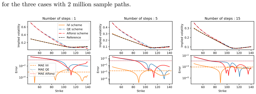
- For Heston option pricing, each step adds only one independent standard Gaussian, and the experiments show accurate ITM/ATM/OTM option prices with 1–5 time steps.
- The scheme has no switching thresholds or stored grids, so it is easy to code and appeared stable in low-sample-path tests.
Reading between the lines
- Because the scheme samples $U$ and $Z$ jointly from a first-passage law, it is naturally suited to payoffs on the whole integrated-variance trajectory, such as Asian-style vol products, rather than only terminal values.
- The same 'simulate the integrated quantity first' idea may extend to other affine processes whose integrated component admits a tractable hitting-time representation; the paper notes that multivariate Wishart-type extensions are not straightforward.
- A natural testable extension is to derive an explicit error bound for the right-endpoint approximation as a function of step size and parameters; such a bound would determine the regimes where the one-step version is reliable.
- For local-stochastic-volatility or rough-Heston settings where the Heston component is simulated alongside an outer model, the scheme's low cost per path and few-step accuracy make it a candidate building block.
Signed reviews
Editorial analysis
A structured set of objections, weighed in public.
Referee Report
Summary. The manuscript proposes a new simulation scheme, called iVi, for the square-root process and the Heston model. The scheme first samples the integrated variance increment U from an Inverse Gaussian distribution whose parameters are obtained by a right-endpoint Euler discretization of the integrated process dynamics, then defines the Brownian-integral increment Z deterministically from U, and finally updates V through the exact drift relation. The main theoretical results are Theorem 1.3 (nonnegativity of the simulated V), Proposition 1.4 (exact first conditional moments for V, U, and Z), Proposition 1.5 and Remark 1.6 (the Inverse Gaussian law arises from an implicit Euler discretization of the Riccati equations), and Remark 1.7 (recovery of known Inverse Gaussian limiting laws in high-mean-reversion and long-maturity regimes). Numerical experiments compare the scheme to the QE scheme of Andersen and the Alfonsi scheme, for variance swaps, volatility swaps, Laplace transforms of integrated variance, and Heston call option prices and implied volatilities, across three calibrated parameter sets. The paper reports high accuracy with as few as one to five time steps. Section 4 states extensions to Volterra/rough Heston settings and refers to a companion paper for convergence proofs.
Significance. If the numerical findings are representative, the iVi scheme is a practically attractive addition to the simulation toolbox: it is parameter-free, simple to implement, preserves nonnegativity, matches first conditional moments exactly, and is competitive with, or better than, established schemes in the tested regimes, especially for short-maturity high-mean-reversion calibrations. The nonnegativity and moment-matching proofs are clean and easily verifiable, and the numerical study is extensive and reproducible in structure. The main limitation is that the accuracy that makes the scheme useful is not established theoretically in this manuscript; the right-endpoint discretization is heuristic, and convergence is deferred to a companion paper. The paper is therefore best read as a numerical-method proposal with strong empirical support rather than as a fully analyzed scheme.
major comments (3)
- [Section 1.1, Eqs. (1.2)-(1.4)] The defining approximation of the scheme is the replacement of the exact integrated dynamics (1.2) by the right-endpoint rule (1.3), which collapses the path of Z_{t_i,·} to its endpoint. There is no local weak-error estimate in the manuscript for this step, and Section 4 explicitly outsources convergence to Abi Jaber and Attal (2025). Because the accuracy claims in Sections 2 and 3 rest on this approximation, the manuscript does not, on its own, prove the scheme's accuracy. Please add a local error bound for the right-endpoint replacement (or state precisely what remains to be proved), or downgrade the claim to an empirical/numerical one.
- [Section 3, Eq. (3.2), Propositions 1.4-1.5] The Heston update (3.2) uses the joint law of (U_{i,i+1}, Z_{i,i+1}) through the term ρ Z_{i,i+1}. Proposition 1.4 only matches first conditional moments, and Proposition 1.5 compares only the marginal Laplace transform of U with the z-argument set to zero. Algorithm 1 makes Ẑ conditionally degenerate given Û, whereas the true Z_{i,i+1} conditional on the single value U_{i,i+1}=u is generally not degenerate, because the path of V inside the interval is not determined by the one integrated value. The numerical tests include ρ = -0.68, -0.70, and -0.9, but the paper gives no bound on the joint weak error, so the reported price accuracy is not guaranteed to persist for, e.g., |ρ| close to 1 or very short maturities. Please analyze the joint-law error or add a systematic stress test over ρ and maturity.
- [Abstract and Remark 1.7] The abstract states that the scheme 'yields the exact limiting Inverse Gaussian distributions' in two regimes. The manuscript does not prove these limiting results; it cites Mechkov (2015), Abi Jaber and De Carvalho (2024), McCrickerd (2019), and Forde and Jacquier (2011). Since the one-step distribution is Inverse Gaussian by construction, the matching is a consequence of known limit theorems. Please either give self-contained proofs of the limits (including the parameters of the limiting laws, which are not stated for the long-maturity case) or reformulate the abstract and Remark 1.7 as 'recovers/reproduces' the known limiting distributions.
minor comments (5)
- [Section 1.1 and Algorithm 1] For α_i=0, the convention IG(0,0)=0 is stated, but the update (0.5) still divides by σ_i; specify the convention for the boundary case, for example when c=0.
- [Proposition 1.5 and Eq. (1.9)] The proposition says that ψ̂ is 'a root' of the quadratic, but only later in Remark 1.6 is it stated that the relevant root has non-positive real part; make this explicit in the proposition.
- [Remark 1.6] The statement that φ̂ corresponds to a trapezoidal discretization is argued only asymptotically; a one-line bound on the remainder would make the remark precise.
- [Section 3, Eq. (3.2)] The independence of N_i from the random variables used in Algorithm 2 is stated in prose; it should be part of the algorithm specification for reproducibility.
- [Introduction and Appendix B] The reference to Duffie, Filipović, and Schachermayer (2003) appears twice in the same sentence; moreover, the branch of the square root in D(u,w) in Eq. (B.2) is not discussed, so the Albrecher et al. (2007) branch choice should be stated for numerical evaluation.
Circularity Check
No significant circularity: the iVi scheme's Inverse Gaussian law follows from an explicit right-endpoint approximation plus Dambis-Dubins-Schwarz time change, and the numerical accuracy claims are benchmarked against external Fourier references; the sole self-citation (companion convergence theorems) is not load-bearing for those claims.
full rationale
The scheme's construction is not circular. Algorithm 1 first defines alpha_i and sigma_i from the model parameters, then samples U from IG(alpha_i, (alpha_i/sigma_i)^2), sets Z=(U-alpha_i)/sigma_i, and updates V by the exact dynamics relation. The Inverse Gaussian law is derived, not assumed: the paper approximates the integral in Proposition 1.1 by the right-endpoint rule, applies Dambis-Dubins-Schwarz to write Z_{s,t} = Wtilde_{U_{s,t}}, and obtains the implicit first-passage equation U = alpha + sigma Wtilde_U, whose solution is an Inverse Gaussian distribution. This is a self-contained mathematical derivation. Proposition 1.4 (first-moment matching) is a consequence of defining alpha_i as the exact conditional mean of U, but the paper treats it only as a sanity check and benchmarks higher moments and option prices against external Fourier/reference values in Sections 2 and 3. Proposition 1.5 and Remark 1.6 restate the same right-endpoint discretization at the level of the Riccati equation; this is a consistency argument, not an input-output circularity. The only self-referential element is Section 4, where theoretical convergence is deferred to Abi Jaber and Attal (2025), a companion paper with overlapping authorship. That self-citation is a completeness gap for the convergence proof, but it is not load-bearing for the paper's empirical accuracy claims, which are supported by independent benchmark comparisons. The lack of an in-paper weak-error bound for the right-endpoint approximation is a correctness risk, not circularity.
Assumptions & free parameters
assumptions (4)
- ad hoc to paper Right-endpoint Euler discretization of the integrated process dynamics and of the Riccati equation is sufficiently accurate for the intended step sizes and parameter regimes.
- standard math Dambis-Dubins-Schwarz theorem: the continuous local martingale Z_{s,*} can be represented as a time-changed Brownian motion.
- ad hoc to paper The Inverse Gaussian law is an adequate conditional proxy for the pair (U_{i,i+1}, Z_{i,i+1}) given V_i.
- domain assumption Known closed-form conditional Laplace transform and Riccati equations for the Heston model (B.1)-(B.3).
Cite this review
Pith. "Pith review of Simulation of square-root processes made simple: applications to the Heston model." pith.science (2026). https://pith.science/paper/3EQTPQBP
@misc{pith2026241211264,
  author       = {Pith},
  title        = {Pith review of: Simulation of square-root processes made simple: applications to the Heston model},
  year         = {2026},
  howpublished = {\url{https://pith.science/paper/3EQTPQBP}},
  note         = {Machine review of arXiv:2412.11264}
}
read the original abstract
We introduce a simple, efficient and accurate nonnegative preserving numerical scheme for simulating the square-root process. The novel idea is to simulate the integrated square-root process first instead of the square-root process itself. Numerical experiments on realistic parameter sets, applied for the integrated process and the Heston model, display high precision with a very low number of time steps. As a bonus, our scheme yields the exact limiting Inverse Gaussian distributions of the integrated square-root process with only one single time-step in two scenarios: (i) for high mean-reversion and volatility-of-volatility regimes, regardless of maturity; and (ii) for long maturities, independent of the other parameters.
Figures


Figures from the paper (7 more)



Forward citations
Cited by 4 Pith papers
-
Diffusion bridge with randomized initial and terminal times and its application to fish migration
A well-posed CIR bridge with time-changed random initial and terminal times models water-temperature-driven Ayu migration and is explored on fish-count and eDNA data.
-
Stochastic partial differential equation model for environmental DNA dynamics in river environments
A stochastic partial differential equation with a delayed source models riverine eDNA from migrating fish, with a closed-form Laplace functional and a nonnegativity-preserving numerical scheme.
-
CIR bridge for modeling of fish migration on sub-hourly scale
A CIR bridge with closed-form mean and variance is proposed and fitted to sub-hourly ayu migration counts, capturing the observed bursty intermittency.
-
Simulating integrated Volterra square-root processes and Volterra Heston models via Inverse Gaussian
An inverse-Gaussian implicit scheme for integrated Volterra square-root processes is proved weakly convergent and shown numerically accurate with very few time steps, including for hyper-rough fractional kernels.
Reference graph
Works this paper leans on
-
[1]
Eduardo Abi Jaber and Elie Attal. Simulating integrated V olterra square-root processes and V olterra H eston models via I nverse G aussian. arXiv preprint arXiv:2504.19885, 2025
arXiv 2025
-
[2]
Reconciling rough volatility with jumps
Eduardo Abi Jaber and Nathan De Carvalho. Reconciling rough volatility with jumps. SIAM Journal on Financial Mathematics, 15 0 (3): 0 785--823, 2024
work page 2024
-
[3]
Hansj \"o rg Albrecher, Philipp Mayer, Wim Schoutens, and Jurgen Tistaert. The little H eston trap. Wilmott, 0 (1): 0 83--92, 2007
work page 2007
-
[4]
On the discretization schemes for the CIR (and B essel squared) processes
Aur \'e lien Alfonsi. On the discretization schemes for the CIR (and B essel squared) processes. Monte Carlo Methods Appl., 11 0 (4): 0 355--384, 2005
work page 2005
-
[5]
Aur \'e lien Alfonsi. High order discretization schemes for the CIR process: application to affine term structure and H eston models. Mathematics of computation, 79 0 (269): 0 209--237, 2010
work page 2010
-
[6]
Simple and efficient simulation of the H eston stochastic volatility model
Leif Andersen. Simple and efficient simulation of the H eston stochastic volatility model. Journal of Computational Finance, 11 0 (3): 0 1--43, 2008
work page 2008
-
[7]
Simulating from the H eston model: A gamma approximation scheme
Jean-Fran c ois B \'e gin, Myl \`e ne B \'e dard, and Patrice Gaillardetz. Simulating from the H eston model: A gamma approximation scheme. Monte Carlo Methods and Applications, 21 0 (3): 0 205--231, 2015
work page 2015
-
[8]
Euler scheme for SDE s with non- L ipschitz diffusion coefficient: strong convergence
Abdel Berkaoui, Mireille Bossy, and Awa Diop. Euler scheme for SDE s with non- L ipschitz diffusion coefficient: strong convergence. ESAIM: Probability and Statistics, 12: 0 1--11, 2008
work page 2008
Show all 32 references
-
[9]
Exact simulation of stochastic volatility and other affine jump diffusion processes
Mark Broadie and \"O zg \"u r Kaya. Exact simulation of stochastic volatility and other affine jump diffusion processes. Operations research, 54 0 (2): 0 217--231, 2006
2006
-
[10]
Simulation schemes for the H eston model with P oisson conditioning
Jaehyuk Choi and Yue Kuen Kwok. Simulation schemes for the H eston model with P oisson conditioning. European Journal of Operational Research, 314 0 (1): 0 363--376, 2024
2024
-
[11]
A theory of the term structure of interest rates
John C Cox, Jonathan E Ingersoll Jr, and Stephen A Ross. A theory of the term structure of interest rates. Econometrica: Journal of the Econometric Society, pages 385--407, 1985
1985
-
[12]
Convergence of discretized stochastic (interest rate) processes with stochastic drift term
Griselda Deelstra and Freddy Delbaen. Convergence of discretized stochastic (interest rate) processes with stochastic drift term. Applied stochastic models and data analysis, 14 0 (1): 0 77--84, 1998
1998
-
[13]
Credit risk: pricing, measurement, and management
Darrell Duffie and Kenneth J Singleton. Credit risk: pricing, measurement, and management. In Credit Risk. Princeton university press, 2012
2012
-
[14]
Affine processes and applications in finance
Darrell Duffie, Damir Filipovi \'c , and Walter Schachermayer. Affine processes and applications in finance. The Annals of Applied Probability, 13 0 (3): 0 984--1053, 2003
2003
-
[15]
The large-maturity smile for the H eston model
Martin Forde and Antoine Jacquier. The large-maturity smile for the H eston model. Finance and Stochastics, 15 0 (4): 0 755--780, 2011
2011
-
[16]
The volatility surface: A Practitioner's Guide
J Gatheral. The volatility surface: A Practitioner's Guide. John Wiley and Sons, Inc, 2011
2011
-
[17]
Gamma expansion of the H eston stochastic volatility model
Paul Glasserman and Kyoung-Kuk Kim. Gamma expansion of the H eston stochastic volatility model. Finance and Stochastics, 15: 0 267--296, 2011
2011
-
[18]
o ngy and Mikl \'o s R \'a sonyi. A note on E uler approximations for SDE s with H \
Istv \'a n Gy \"o ngy and Mikl \'o s R \'a sonyi. A note on E uler approximations for SDE s with H \"o lder continuous diffusion coefficients. Stochastic processes and their applications, 121 0 (10): 0 2189--2200, 2011
2011
-
[19]
A closed-form solution for options with stochastic volatility with applications to bond and currency options
Steven L Heston. A closed-form solution for options with stochastic volatility with applications to bond and currency options. The review of financial studies, 6 0 (2): 0 327--343, 1993
1993
-
[20]
Convergence of M onte C arlo simulations involving the mean-reverting square root process
Desmond J Higham and Xuerong Mao. Convergence of M onte C arlo simulations involving the mean-reverting square root process. Journal of Computational Finance, 8 0 (3): 0 35--61, 2005
2005
-
[21]
Fast strong approximation M onte C arlo schemes for stochastic volatility models
Christian Kahl and Peter J \"a ckel. Fast strong approximation M onte C arlo schemes for stochastic volatility models. Quantitative Finance, 6 0 (6): 0 513--536, 2006
2006
-
[22]
Weak approximation of CKLS and CEV processes by discrete random variables
Gytenis Lileika and Vigirdas Mackevi c ius. Weak approximation of CKLS and CEV processes by discrete random variables. Lithuanian Mathematical Journal, 60: 0 208--224, 2020
2020
-
[23]
On spatially irregular ordinary differential equations and a pathwise volatility modelling framework
Ryan McCrickerd. On spatially irregular ordinary differential equations and a pathwise volatility modelling framework. arXiv preprint arXiv:1902.01673, 2019
1902 arXiv
-
[24]
Fast-reversion limit of the H eston model
Serguei Mechkov. Fast-reversion limit of the H eston model. Available at SSRN 2418631, 2015
2015
-
[25]
Generating random variates using transformations with multiple roots
John R Michael, William R Schucany, and Roy W Haas. Generating random variates using transformations with multiple roots. The American Statistician, 30 0 (2): 0 88--90, 1976
1976
-
[26]
First order strong approximations of scalar SDE s defined in a domain
Andreas Neuenkirch and Lukasz Szpruch. First order strong approximations of scalar SDE s defined in a domain. Numerische Mathematik, 128: 0 103--136, 2014
2014
-
[27]
Efficient simulation of the double H eston model
Dylan Possama \" and Pierre Gauthier. Efficient simulation of the double H eston model. The IUP Journal of Computational Mathematics, 4 0 (3): 0 23--73, 2011
2011
-
[28]
Continuous martingales and B rownian motion , volume 293
Daniel Revuz and Marc Yor. Continuous martingales and B rownian motion , volume 293. Springer Science & Business Media, 2013
2013
-
[29]
Laplace transforms and suprema of stochastic processes
Klaus Sch \"u rger. Laplace transforms and suprema of stochastic processes. Advances in finance and stochastics: essays in honour of Dieter Sondermann, pages 285--294, 2002
2002
-
[30]
Low-bias simulation scheme for the H eston model by I nverse G aussian approximation
Shu Tong Tse and Justin WL Wan. Low-bias simulation scheme for the H eston model by I nverse G aussian approximation. Quantitative finance, 13 0 (6): 0 919--937, 2013
2013
-
[31]
Efficient, almost exact simulation of the H eston stochastic volatility model
Alexander Van Haastrecht and Antoon Pelsser. Efficient, almost exact simulation of the H eston stochastic volatility model. International Journal of Theoretical and Applied Finance, 13 0 (01): 0 1--43, 2010
2010
-
[32]
A simple and accurate simulation approach to the H eston model
Jianwei Zhu. A simple and accurate simulation approach to the H eston model. Journal of Derivatives, 18 0 (4): 0 26, 2011
2011
Reviewed August 11, 2026 · model on record in the stance chip above.
Discussion (0). Continue with ORCID to comment.