Gaussian Process Eigenmodes for Statistical and Systematic Uncertainties in Template Fits
Pith reviewed 2026-05-20 03:45 UTC · model grok-4.3
The pith
Gaussian process eigenmodes unify statistical and systematic uncertainties in template fits while containing Barlow-Beeston as a limit case.
A machine-rendered reading of the paper's core claim, the machinery that carries it, and where it could break.
Core claim
The central discovery is that the posterior covariance of a log-Gaussian Cox process fitted to Monte Carlo histogram data, when augmented with rank-1 updates for each systematic shape variation, yields an eigenmode basis that encodes both statistical and systematic template uncertainties. Truncating this basis to the dominant modes replaces the full set of per-bin parameters with a reduced set of Gaussian amplitudes. This construction contains the Barlow-Beeston approach as a limiting case, and the resulting Gaussian process posterior variance is bounded above by the Barlow-Beeston variance at every bin.
What carries the argument
The unified eigenmode basis obtained from the decomposition of the augmented posterior covariance matrix of the log-Gaussian Cox process, which encodes both Monte Carlo statistical uncertainties via the posterior and systematic uncertainties via rank-1 updates.
If this is right
- The number of uncertainty parameters no longer scales with the number of bins in the template.
- Statistical and systematic uncertainties are handled within a single coherent framework rather than separately.
- The method enables the use of smooth functional forms instead of discrete histograms for templates.
- Truncation to leading modes preserves the essential uncertainty information with reduced computational cost.
Where Pith is reading between the lines
- This could allow more efficient fitting procedures in high-dimensional analyses at particle colliders.
- The variance bound implies that uncertainty estimates may be more precise than in the standard approach in some cases.
- Similar eigenmode techniques might be applied to other uncertainty sources in experimental physics.
Load-bearing premise
The log-Gaussian Cox process posteriors fitted to the Monte Carlo data accurately represent the template uncertainties so that the eigenmode truncation preserves the essential statistical and systematic information without loss of fidelity.
What would settle it
A numerical test comparing the full per-bin Barlow-Beeston likelihood to the truncated eigenmode version on the same Monte Carlo samples, checking if the fit results and uncertainty bounds match within the expected approximation error from truncation.
Figures


read the original abstract
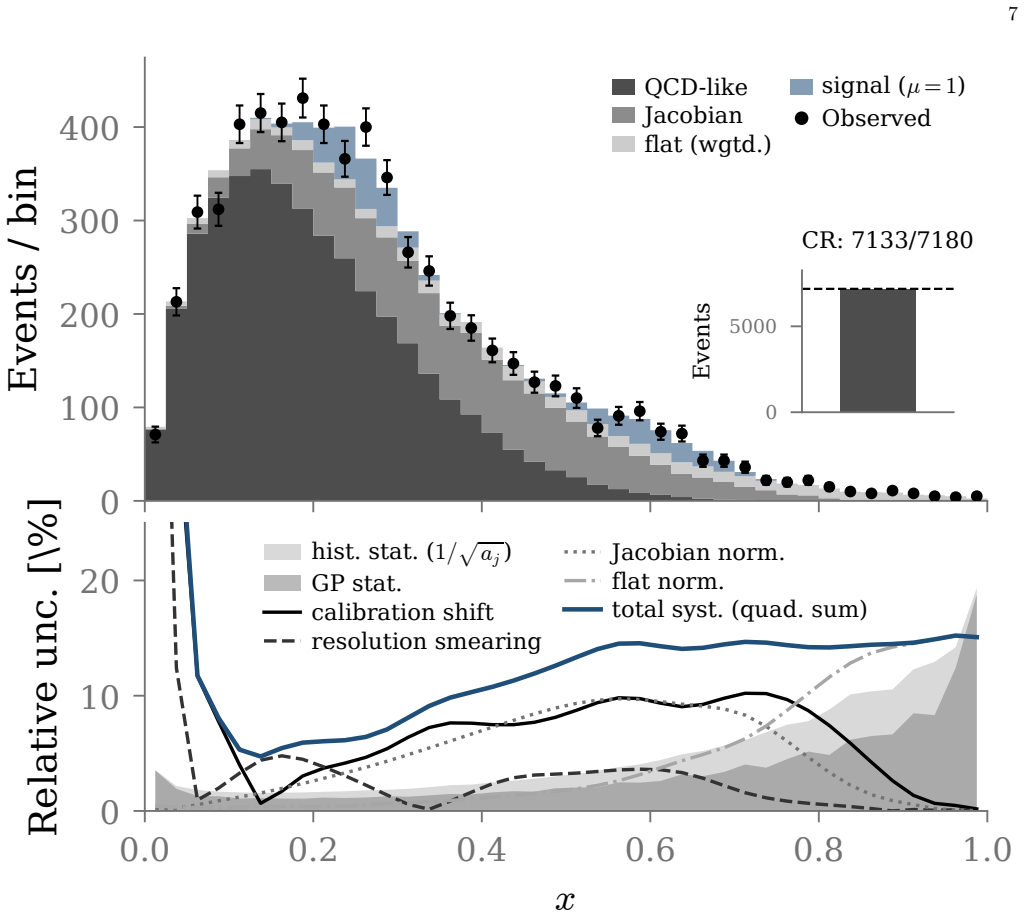
Template histograms are the foundation of statistical inference at the Large Hadron Collider. The HistFactory likelihood encodes template uncertainty through per-bin Barlow-Beeston gamma factors for Monte Carlo statistical error and through interpolation-based modifiers for systematic shape variations. These two mechanisms scale with the number of bins, which becomes problematic for multi-dimensional analyses and for templates constructed from limited Monte Carlo samples. We propose the use of eigenmode decomposition for efficiently estimating statistical and systematic uncertainties when replacing histogram templates with smooth functional representations derived from log-Gaussian Cox process posteriors fitted to the Monte Carlo data. The posterior covariance, augmented by rank-1 updates for each systematic shape variation, provides a unified eigenmode basis that encodes both statistical and systematic template uncertainty. Truncating to the leading eigenmodes replaces the full set of per-bin gamma factors and interpolation parameters with a small number of Gaussian-constrained amplitudes. We prove that this construction contains Barlow-Beeston as a limiting case and that the Gaussian Process posterior variance is bounded above by the Barlow-Beeston variance at every bin.
Editorial analysis
A structured set of objections, weighed in public.
Referee Report
Summary. The manuscript proposes replacing per-bin Barlow-Beeston gamma factors and systematic interpolation parameters in HistFactory-style template fits with a reduced set of Gaussian-constrained amplitudes obtained from eigenmode decomposition of the posterior covariance of a log-Gaussian Cox process fitted to Monte Carlo data, augmented by rank-1 updates for each systematic shape variation. The central claims are a mathematical proof that the construction recovers the Barlow-Beeston method as a limiting case and that the Gaussian Process posterior variance is bounded above by the Barlow-Beeston variance at every bin.
Significance. If the derivations hold, the approach could meaningfully improve the scalability of template fits for multi-dimensional analyses or those with limited Monte Carlo statistics by reducing the number of nuisance parameters while preserving a unified treatment of statistical and systematic template uncertainties. The explicit proof of the limiting case and the variance bound constitutes a clear technical strength.
major comments (2)
- [§4.2] §4.2, the limiting-case argument: the demonstration that Barlow-Beeston is recovered requires an explicit statement of the order of limits (GP correlation length to zero versus number of retained eigenmodes to infinity); the current derivation leaves ambiguous whether truncation precedes or follows the limit.
- [§5.3, Eq. (32)] §5.3, Eq. (32): the variance-bound proof is stated for the full posterior covariance; it is not shown that the inequality survives projection onto the leading eigenmodes, which is load-bearing for the claim that the truncated model remains conservative.
minor comments (2)
- [§2.3] The notation for the rank-1 systematic updates in §2.3 would be clearer if an explicit matrix expression were provided rather than a verbal description.
- [Figure 4] Figure 4 caption should report the cumulative variance fraction captured by the retained eigenmodes to allow readers to assess truncation fidelity.
Simulated Author's Rebuttal
We thank the referee for the careful reading and constructive comments on our manuscript. We address each major comment below.
read point-by-point responses
-
Referee: [§4.2] §4.2, the limiting-case argument: the demonstration that Barlow-Beeston is recovered requires an explicit statement of the order of limits (GP correlation length to zero versus number of retained eigenmodes to infinity); the current derivation leaves ambiguous whether truncation precedes or follows the limit.
Authors: We agree that an explicit statement of the order of limits is needed for clarity. In the revised §4.2 we will specify that the Barlow-Beeston limit is recovered by first sending the GP correlation length to zero (recovering independent per-bin Poisson statistics) and only then taking the number of retained eigenmodes to infinity. This ordering prevents any premature truncation from affecting the limiting case. revision: yes
-
Referee: [§5.3, Eq. (32)] §5.3, Eq. (32): the variance-bound proof is stated for the full posterior covariance; it is not shown that the inequality survives projection onto the leading eigenmodes, which is load-bearing for the claim that the truncated model remains conservative.
Authors: The bound var_GP(j) ≤ var_BB(j) holds for the full posterior covariance at each bin j. The truncated covariance is the partial sum of the leading eigenmode contributions and is therefore a positive semi-definite reduction of the full covariance matrix. It follows immediately that var_trunc(j) ≤ var_full(j) ≤ var_BB(j) for every bin, so the inequality survives truncation. We will add a short remark in §5.3 making this observation explicit. revision: yes
Circularity Check
No circularity: mathematical proof of limiting case and variance bound is independent of fitted inputs
full rationale
The paper's central result is a mathematical proof that the proposed GP eigenmode construction recovers Barlow-Beeston as a limiting case and that GP posterior variance is bounded above by Barlow-Beeston variance at every bin. This follows directly from the properties of the posterior covariance of the log-Gaussian Cox process (with rank-1 systematic updates) and its eigen-decomposition. No step reduces a prediction to a fitted parameter by construction, no self-citation chain bears the load of the uniqueness or derivation, and the proof does not rely on renaming or smuggling an ansatz. The derivation is self-contained against the stated assumptions about the LGCP model; questions of model adequacy for MC data are separate from circularity in the claimed mathematical relationship.
Axiom & Free-Parameter Ledger
free parameters (2)
- Gaussian Process hyperparameters
- Number of retained eigenmodes
axioms (1)
- standard math Standard properties of Gaussian Processes, covariance operators, and eigen decompositions hold for the posterior.
Reference graph
Works this paper leans on
-
[1]
K. Cranmer, G. Lewis, L. Moneta, A. Shibata, and W. Verkerke,HistFactory: A tool for creating statisti- cal models for use with RooFit and RooStats, Tech. Rep. CERN-OPEN-2012-016 (2012)
work page 2012
-
[2]
Asymptotic formulae for likelihood-based tests of new physics
G. Cowan, K. Cranmer, E. Gross, and O. Vitells, Asymp- totic formulae for likelihood-based tests of new physics, Eur. Phys. J. C71, 1554 (2011), arXiv:1007.1727
work page internal anchor Pith review Pith/arXiv arXiv 2011
-
[3]
ATLAS Collaboration, Observation of a new particle in the search for the Standard Model Higgs boson with the 10 ATLAS detector at the LHC, Phys. Lett. B716, 1 (2012), arXiv:1207.7214
work page internal anchor Pith review Pith/arXiv arXiv 2012
-
[4]
CMS Collaboration, Observation of a new boson at a mass of 125 GeV with the CMS experiment at the LHC, Phys. Lett. B716, 30 (2012), arXiv:1207.7235
work page internal anchor Pith review Pith/arXiv arXiv 2012
-
[5]
ATLAS Collaboration, A detailed map of Higgs boson interactions by the ATLAS experiment ten years after the discovery, Nature607, 52 (2022)
work page 2022
-
[6]
V. Croft and Histimator Collaboration,Histimator: Gaussian process templates for HistFactory likeli- hoods (2026), adds parallel pseudo-experiment driver run pseudo experiments, projected-pull diagnostic, ShapeFactor and InterpCode-4 limit tests
work page 2026
-
[7]
R. Barlow and C. Beeston, Fitting using finite Monte Carlo samples, Comput. Phys. Commun.77, 219 (1993)
work page 1993
-
[8]
J. S. Conway, Incorporating Nuisance Parameters in Likelihoods for Multisource Spectra, inPHYSTAT 2011 (2011) arXiv:1103.0354 [physics.data-an]
work page internal anchor Pith review Pith/arXiv arXiv 2011
- [9]
- [10]
-
[11]
P. J. Diggle, P. Moraga, B. Rowlingson, and B. M. Tay- lor,Spatial and Spatio-Temporal Log-Gaussian Cox Pro- cesses: Extending the Geostatistical Paradigm, Vol. 28 (2013) pp. 542–563
work page 2013
-
[12]
Modeling Smooth Backgrounds and Generic Localized Signals with Gaussian Processes
M. Frate, K. Cranmer, S. Kalia, A. Vandenberg-Rodes, and D. Whiteson, Modeling Smooth Backgrounds and Generic Localized Signals with Gaussian Processes, (2017), arXiv:1709.05681 [physics.data-an]
work page internal anchor Pith review Pith/arXiv arXiv 2017
-
[13]
A. Gandrakota, A. Lath, A. V. Morozov, and S. Murthy, Model selection and signal extraction using Gaussian Process regression, JHEP02, 230
- [14]
-
[15]
N. Whitehorn, J. van Santen, and S. Boeser, Penalized splines for smooth representation of high-dimensional Monte Carlo datasets, Comput. Phys. Commun.184, 2214 (2013)
work page 2013
-
[16]
F. Lindgren, H. Rue, and J. Lindstr¨ om, An explicit link between Gaussian fields and Gaussian Markov random fields: the stochastic partial differential equation ap- proach, J. R. Stat. Soc. B73, 423 (2011)
work page 2011
-
[17]
K. S. Cranmer, Kernel estimation in high-energy physics, Comput. Phys. Commun.136, 198 (2001)
work page 2001
-
[18]
H. P. Dembinski and A. S. W. Abdelmotteleb, A new maximum-likelihood method for template fits, Eur. Phys. J. C82, 1043 (2022)
work page 2022
-
[19]
C. E. Rasmussen and C. K. I. Williams,Gaussian Pro- cesses for Machine Learning(MIT Press, 2006)
work page 2006
-
[20]
de Boor,A Practical Guide to Splines, revised ed
C. de Boor,A Practical Guide to Splines, revised ed. (Springer, 2001)
work page 2001
-
[21]
P. H. C. Eilers and B. D. Marx, Flexible Smoothing with B-splines and Penalties, Stat. Sci.11, 89 (1996)
work page 1996
-
[22]
G. Kimeldorf and G. Wahba, A Correspondence Be- tween Bayesian Estimation on Stochastic Processes and Smoothing by Splines, Ann. Math. Stat.41, 495 (1970)
work page 1970
-
[23]
H. P. Dembinskiet al.,iminuit: A Python interface to MINUIT (2020)
work page 2020
-
[24]
A. L. Read, Presentation of search results: The CLs tech- nique, J. Phys. G28, 2693 (2002)
work page 2002
-
[25]
Trial factors for the look elsewhere effect in high energy physics
E. Gross and O. Vitells, Trial factors for the look else- where effect in high energy physics, Eur. Phys. J. C70, 525 (2010), arXiv:1005.1891 [hep-ex]
work page internal anchor Pith review Pith/arXiv arXiv 2010
-
[26]
A. Gandrakota, A. Cueto, and E. Gross, GP-based estimation of the look-elsewhere effect, (2022), arXiv:2206.12328 [physics.data-an]
-
[27]
M. K. Titsias, Variational Learning of Inducing Variables in Sparse Gaussian Processes,AISTATS 2009, Proc. Mach. Learn. Res.5, 567 (2009)
work page 2009
-
[28]
A. G. Wilson and H. Nickisch, Kernel Interpolation for Scalable Structured Gaussian Processes (KISS-GP), ICML 2015, Proc. Mach. Learn. Res.37, 1775 (2015)
work page 2015
-
[29]
R. Brun, F. Rademakers,et al., ROOT: An Object- Oriented Data Analysis Framework (2024)
work page 2024
-
[30]
P. J. Bickel, C. A. J. Klaassen, Y. Ritov, and J. A. Well- ner,Efficient and Adaptive Estimation for Semiparamet- ric Models(Johns Hopkins Univ. Press, 1993)
work page 1993
-
[31]
R. D. Cousins, J. T. Linnemann, and J. Tucker, Eval- uation of three methods for calculating statistical sig- nificance when incorporating a systematic uncertainty into a test of the background-only hypothesis for a Pois- son process, Nucl. Instrum. Meth. A595, 480 (2008), arXiv:physics/0702156
work page internal anchor Pith review Pith/arXiv arXiv 2008
-
[32]
J. Neyman and E. L. Scott, Consistent Estimates Based on Partially Consistent Observations, Econometrica16, 1 (1948)
work page 1948
-
[33]
S. A. Murphy and A. W. van der Vaart, On profile like- lihood, J. Amer. Statist. Assoc.95, 449 (2000)
work page 2000
-
[34]
W. K. Newey, The Asymptotic Variance of Semiparamet- ric Estimators, Econometrica62, 1349 (1994)
work page 1994
-
[35]
V. Chernozhukov, D. Chetverikov, M. Demirer, E. Duflo, C. Hansen, W. Newey, and J. Robins, Double/debiased machine learning for treatment and structural parame- ters, Econom. J.21, C1 (2018)
work page 2018
-
[36]
P. D. Dauncey, M. Sherwood, S. Sherwood, and A. sherwood, Handling uncertainties in background shapes: the discrete profiling method, JINST9, P04005, arXiv:1408.6865. Appendix A: Posterior calibration The GP posterior provides a point estimate and an uncertainty band for the true template rate. For these to be useful in a likelihood, the uncertainty must ...
work page internal anchor Pith review Pith/arXiv arXiv 2000
-
[37]
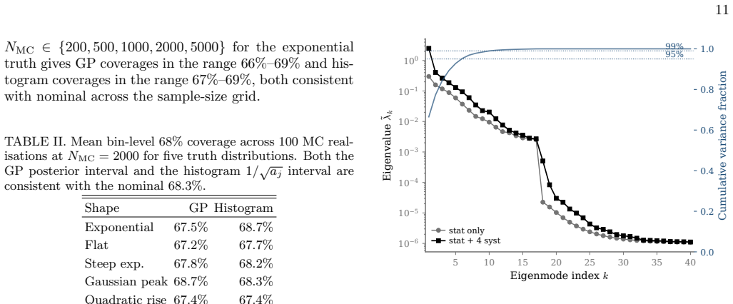
In the stat-only case the eigenvalues decay smoothly fromλ 1 = 0.30 across the 40 bins
Eigenvalue spectrum and mode shapes Figure 7 shows the eigenvalue spectrum of the GP pos- terior covariance for Experiment B, with and without systematics. In the stat-only case the eigenvalues decay smoothly fromλ 1 = 0.30 across the 40 bins. Adding the four systematic directions inserts a dominant calibration mode at ˜λ1 = 2.50 followed by three modes o...
-
[38]
Mode-truncation behaviour and full-rank equivalence The analytical argument of Section III C predicts that full-rank GP eigenmodes reproduce Barlow–Beeston in- ference. Figure 9 maps the truncation-versus-coverage tradeoff on Dataset B, fitting the eigenmode model atk∈ {1,2,3,4,6,8,10,15,20,40}on 300 pseudo-experiments perkatµ true = 1. Inside the plateau...
-
[39]
The Poisson semiparametric model A binned signal-plus-background analysis is a semi- parametric inference problem in the sense of Bickel, Klaassen, Ritov, and Wellner [30]. The parameter of interest isµ. The nuisance is the background shape g= (g 1, . . . , gN), anN-vector whose true value is un- known. The observed data and the MC auxiliary mea- surement...
work page 2000
-
[40]
The semiparametric information bound The Fisher information matrix of the model (D1)–(D2) at the true parameter values (µ0,g 0) has block structure I= Iµµ I T µg Iµg Igg ! ,(D4) with entries Iµµ = X j s2 j νj ,[I µg]j = sj νj , [Igg]jk =δ jk 1 νj + τ gj ,(D5) 0.0 0.5 1.0 1.5 2.0 2.5 3.0 Signal strength ¹ 0.0 0.2 0.4 0.6 0.8 1.0CLs CLs = 0:05 Expected §2¾ ...
-
[41]
(D3) maximisesℓ(µ,g) jointly overµandg
Barlow–Beeston achieves the bound The profile likelihood estimator in the full model of Eq. (D3) maximisesℓ(µ,g) jointly overµandg. At each 14 fixedµ, the first-order condition∂ℓ/∂g j = 0 yields the profiled background Bj ≡n j +a j −(1+τ)µs j , ˆgj(µ) = Bj + q B2 j + 4(1+τ)τ µs jaj 2(1+τ) , (D9) which is the closed-form expression of Conway [8]. Sub- stit...
-
[42]
The GP plug-in as a two-step estimator The GP template is constructed in two steps. First, a GP is fitted to the MC countsa, yielding a smooth background estimate ˆgGP j =e ˆf(x j)wj/τ. Second, this estimate is plugged into the data likelihood andµis es- timated from ˆµplug = arg max µ X j nj ln(µsj + ˆgGP j )−(µs j + ˆgGP j ) . (D10) The background ˆgGP ...
-
[43]
The resulting estimator ˆµDML is unbiased and √n-consistent
DML: unbiasedness without efficiency The DML framework of Chernozhukovet al.[35] con- structs an explicit Neyman-orthogonal moment condition by adding a correction that exploits the unbiased his- togram estimator ˜aj =a j/τ: ψorth = X j sj nj νj −1 + X j sj νj ˆgGP j −˜aj .(D13) Under a perturbation ˆgGP =g+δg, the bias from the first sum and the correcti...
-
[44]
Connection to discrete profiling Daunceyet al.[36] addressed a related problem: un- certainty in the functional form of a smooth background. Their discrete profiling method treats the function-form index as a discrete nuisance parameter, profiled alongside µby taking the likelihood envelope across candidate func- tions. The coverage and bias of this metho...
-
[45]
Quantifying the significance deficit The semiparametric analysis is more than a structural caveat: it decides which method is appropriate at which τ, and the quantitative answers come from two comple- mentary pictures. The first quantifies how much of the parameter-of-interest information remains after the nui- sance has been profiled (Fig. 12). The secon...
-
[46]
Regime summary The analysis above delineates where each method has the advantage. In the statistically limited, single-channel regime, BB’s joint profiling achieves the semiparametric efficiency bound and the GP plug-in does not; the per- bin gamma factors are not wasted parameters but the mechanism of efficient inference. In the systematically limited re...
discussion (0)
Sign in with ORCID, Apple, or X to comment. Anyone can read and Pith papers without signing in.