Scientific Logicality Enriched Methodology for LLM Reasoning: A Practice in Physics
Pith reviewed 2026-05-20 15:06 UTC · model grok-4.3
The pith
Enriching LLM training with scientific logicality criteria improves reasoning validity and performance on physics problems.
A machine-rendered reading of the paper's core claim, the machinery that carries it, and where it could break.
Core claim
By defining assessment criteria for scientific logicality and using logicality-guided sampling to construct training data from physics problems in the literature, the authors show that training on this data raises the logical faithfulness of LLM reasoning steps and that the resulting logicality is essential for successfully solving scientific problems.
What carries the argument
Scientific logicality-enriched methodology, consisting of assessment criteria that judge the rational validity of reasoning steps and data sampling methods that select examples exhibiting strong logicality for guided training.
If this is right
- The constructed dataset raises scientific logicality scores in reasoning outputs from three different LLMs.
- Higher logicality directly contributes to better performance on scientific problem-solving tasks.
- The methodology works with physics as a test case that features varied logical structures and formalisms.
- Both logical faithfulness and overall task accuracy increase when training emphasizes step-by-step rational validity.
Where Pith is reading between the lines
- The same criteria and sampling approach could be adapted to build training sets for other sciences such as chemistry or biology.
- Models trained this way may produce fewer invalid intermediate steps when deriving equations or analyzing experimental data.
- Combining logicality-guided data with existing chain-of-thought methods might produce further gains on multi-step problems.
- Testing the trained models on problems drawn from sources outside the original literature would reveal whether the gains generalize.
Load-bearing premise
The authors' assessment criteria for scientific logicality measure a genuine and independent feature of valid reasoning rather than simply reflecting patterns in the selected training examples.
What would settle it
Training the same LLMs on the new dataset and then evaluating them on held-out physics problems yields no measurable gain in either expert-rated logical consistency of reasoning chains or final answer accuracy compared with baseline training.
Figures


read the original abstract
With the continuous advancement of reasoning abilities in Large Language Models (LLMs), their application to scientific reasoning tasks has gained significant research attention. Current research primarily emphasizes boosting LLMs' performance on scientific QA benchmarks by training on larger, more comprehensive datasets with extended reasoning chains. However, these approaches neglect the essence of the scientific reasoning process -- logicality, which is the rational foundation to ensure the validity of reasoning steps leading to reliable conclusions. In this work, we make the first systematic investigation into the internal logicality underlying LLM scientific reasoning, and develop a scientific logicality-enriched methodology, including a set of assessment criteria and data sampling methods for logicality-guided training, to improve the logical faithfulness as well as task performance. Further, we take physics, characterized by its diverse logical structures and formalisms, as an exemplar discipline to practise the above methodology. For data construction, we extract scientific problems from academic literature and sample a high-quality dataset exhibiting strong logicality. Experiments based on three different backbone LLMs reveal that: 1) the training data we constructed can effectively improve the scientific logicality in LLM reasoning; and 2) the enriched scientific logicality plays a critical role in solving scientific problems. Code is available at \href{https://github.com/ScienceOne-AI/PhysLogic}{https://github.com/ScienceOne-AI/PhysLogic}.
Editorial analysis
A structured set of objections, weighed in public.
Referee Report
Summary. The paper claims to make the first systematic investigation into the internal logicality underlying LLM scientific reasoning. It develops assessment criteria and logicality-guided data sampling methods to construct a high-quality training dataset by extracting and selecting scientific problems from academic literature that exhibit strong logicality. Using physics as the exemplar domain, experiments on three backbone LLMs are reported to show that the constructed training data effectively improves scientific logicality in LLM reasoning and that this enriched logicality plays a critical role in solving scientific problems.
Significance. If the central claims hold under rigorous, non-circular evaluation, the work could provide a useful framework for curating training data that emphasizes logical structure and formalisms rather than scale alone, with potential relevance for domain-specific reasoning in the sciences. The open-sourced code at the provided GitHub link is a positive contribution to reproducibility.
major comments (2)
- [Abstract and Experiments] Abstract and Experiments section: The abstract asserts positive results on three LLMs yet supplies no numbers, baselines, error bars, or description of how logicality was scored; the full paper must supply these quantitative details (including exact metrics, comparison models, and statistical tests) so that the two main experimental claims can be verified against the stated methodology.
- [Methodology] Methodology section: Logicality is defined internally by the authors and used both to filter/select the training data and to measure post-training success. This creates a circularity risk for the central claim that the enriched logicality improves reasoning soundness. The paper should add either an external pre-existing benchmark or a blind domain-expert evaluation using a separate rubric to demonstrate that measured gains reflect genuine improvements rather than better alignment with the authors' own labeling scheme.
minor comments (2)
- [Introduction] Clarify in the introduction how the proposed logicality criteria differ from existing notions of step-wise deduction or formal verification in the LLM reasoning literature.
- [Figures] Ensure all figures showing reasoning traces include explicit annotations for the logicality criteria being illustrated.
Simulated Author's Rebuttal
We thank the referee for the constructive comments and the opportunity to revise our manuscript. We address each major comment below and have updated the paper accordingly to improve its rigor and clarity.
read point-by-point responses
-
Referee: [Abstract and Experiments] Abstract and Experiments section: The abstract asserts positive results on three LLMs yet supplies no numbers, baselines, error bars, or description of how logicality was scored; the full paper must supply these quantitative details (including exact metrics, comparison models, and statistical tests) so that the two main experimental claims can be verified against the stated methodology.
Authors: We agree that quantitative details are crucial for the verifiability of our results. The revised manuscript will feature an updated abstract that reports specific numerical improvements in both logicality and task performance for the three backbone LLMs. In the Experiments section, we will provide comprehensive tables including exact metrics, baseline comparisons, error bars, a detailed description of the logicality scoring procedure, and results from statistical significance tests. revision: yes
-
Referee: [Methodology] Methodology section: Logicality is defined internally by the authors and used both to filter/select the training data and to measure post-training success. This creates a circularity risk for the central claim that the enriched logicality improves reasoning soundness. The paper should add either an external pre-existing benchmark or a blind domain-expert evaluation using a separate rubric to demonstrate that measured gains reflect genuine improvements rather than better alignment with the authors' own labeling scheme.
Authors: We thank the referee for highlighting this important methodological consideration. To address the risk of circularity, the revised paper will include performance evaluations on an external pre-existing scientific reasoning benchmark. In addition, we will report the outcomes of a blind evaluation conducted by domain experts employing a distinct rubric for assessing reasoning soundness. These measures will help substantiate that the observed gains represent authentic advancements rather than artifacts of our internal criteria. revision: yes
Circularity Check
Internally defined logicality criteria used for both data sampling and evaluation create circularity risk in claimed improvements.
specific steps
-
fitted input called prediction
[Abstract]
"For data construction, we extract scientific problems from academic literature and sample a high-quality dataset exhibiting strong logicality. Experiments based on three different backbone LLMs reveal that: 1) the training data we constructed can effectively improve the scientific logicality in LLM reasoning; and 2) the enriched scientific logicality plays a critical role in solving scientific problems."
The logicality assessment criteria are first used to filter/select the training data (high-logicality subset), after which the same criteria are applied to quantify post-training gains in scientific logicality. The reported improvement is therefore aligned with the selection filter by design rather than demonstrating an independent gain in reasoning validity.
full rationale
The paper defines its own assessment criteria for scientific logicality, uses those criteria to sample and construct a high-quality training dataset of problems exhibiting strong logicality, then trains LLMs and reports that the data improves scientific logicality (measured via the same criteria) and task performance. This creates a closed loop where the central experimental result is an improvement on the authors' own filtering metric rather than an externally anchored property of reasoning. No independent benchmark, blind expert rubric, or pre-existing logicality standard is invoked to break the loop. The derivation chain for the key claims therefore reduces to the input selection process by construction.
Axiom & Free-Parameter Ledger
axioms (1)
- domain assumption Scientific logicality is a distinct, assessable property of reasoning steps that can be improved by targeted data selection.
Lean theorems connected to this paper
-
IndisputableMonolith/Foundation/ArithmeticFromLogic.leanLogicNat recovery and embed_strictMono echoes?
echoesECHOES: this paper passage has the same mathematical shape or conceptual pattern as the Recognition theorem, but is not a direct formal dependency.
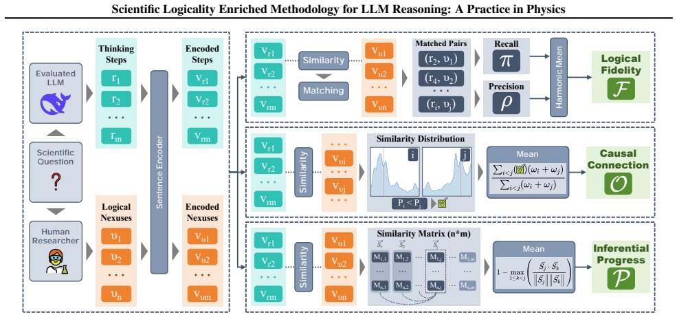
We design criteria with three complementary dimensions... Logical Fidelity F... Causal Connection O... Inferential Progress P... using sentence encoder embeddings VN and VR, greedy matching, positional centroids Pi, and novelty 1−max cosine similarity of similarity vectors Sj.
-
IndisputableMonolith/Foundation/LogicAsFunctionalEquation.leanSatisfiesLawsOfLogic and Translation Theorem unclear?
unclearRelation between the paper passage and the cited Recognition theorem.
We extract scientific problems from academic literature and sample a high-quality dataset exhibiting strong logicality... two SFT data sampling methods, based on distillation and reasoning style transfer.
What do these tags mean?
- matches
- The paper's claim is directly supported by a theorem in the formal canon.
- supports
- The theorem supports part of the paper's argument, but the paper may add assumptions or extra steps.
- extends
- The paper goes beyond the formal theorem; the theorem is a base layer rather than the whole result.
- uses
- The paper appears to rely on the theorem as machinery.
- contradicts
- The paper's claim conflicts with a theorem or certificate in the canon.
- unclear
- Pith found a possible connection, but the passage is too broad, indirect, or ambiguous to say the theorem truly supports the claim.
Reference graph
Works this paper leans on
-
[1]
1.") and ending with the score in parentheses
Calculate the difference in coefficients of thermal expansion: \alpha_{\text{torsion}}−\alpha_{\text{sub}} = 3.5 \times 10^{−6} \,^{\circ}\text{C}^{−1} (10 points) # Output Format Please output these scoring points directly in English text, one point per line, each starting with an ordered list number (e.g., "1.") and ending with the score in parentheses ...
-
[2]
Define the deviationδC=C−1/2and identifyy 1 = √1−2C≈ p |2δC|near the BH limit. (10 points)
- [3]
-
[4]
Apply coordinate transformationx= 1−yto find the singular surfacex 0 =−κ≈1−3 p 2|δC|and surface coordinate x1 = 1−y 1 ≈1− p 2|δC|. (15 points)
- [5]
-
[6]
Formulate the tidal perturbation as a Riccati equation in thex-coordinate, noting coefficient singularities atx0 due to pressure divergence. (15 points)
-
[7]
Derive the solution’s exponential suppression nearx0:∝exp(−b/ p |δC|)forb >0, using WKB-like asymptotics or Frobenius analysis. (20 points)
-
[8]
Evaluatehat the surface (x 1) and substitute into thek2 formula to confirmk2 ∝exp(−b/|δC|), rejecting options A, B, and D. (15 points) 32 Scientific Logicality Enriched Methodology for LLM Reasoning: A Practice in Physics J.2. Expression Computation Below is an example of an expression computation problem: •Difficulty:PhD student •Subdomain:mathematical p...
-
[9]
Rearrange terms to isolate the square root: 1− θ 4dβ −κ≤θ I u,d (1,−1) √ 2 √κ
-
[10]
Define substitutions: Letx= √κ(sox≥0), and set: A=θ I u,d (1,−1) √ 2 , B= 1− θ 4dβ The inequality becomes: B−x 2 ≤Ax
-
[11]
Form a quadratic inequality: Rearrange to: x2 +Ax−B≥0 This quadratic inequality holds whenx≥ −A+ √ A2+4B 2 (consideringx≥0and the quadratic’s positive root)
-
[12]
Substitute back: Sinceκ=x 2, the lower bound is: κ≥ −A+ √ A2 + 4B 2 !2 ReplacingAandB: κ≥ −θ Iu,d (1,−1)√ 2 + vuut θ Iu,d (1,−1)√ 2 !2 + 4 1− θ 4dβ 2 2 33 Scientific Logicality Enriched Methodology for LLM Reasoning: A Practice in Physics
-
[13]
Simplify the expression: The term inside the square root simplifies as: θ I u,d (1,−1) √ 2 2 + 4− θ dβ = θ2(I u,d (1,−1))2 2 + 4− θ dβ Thus: κ≥ s θ2(Iu,d (1,−1))2 2 + 4− θ dβ −θ Iu,d (1,−1)√ 2 2 2 This is the lower bound for the nearest-neighbor connection probabilityκ. κ≥ vuut θ2 I u,d (1,−1) 2 2 + 4− θ dβ −θ I u,d (1,−1)...
-
[14]
Rearrange the given inequality to isolate constant andκterms: move θ 4dβ to the left andκto the right, yielding1−κ− θ 4dβ ≤ θ Iu,d (1,−1)√ 2 √κ. (10 points)
-
[15]
Substitutex= √κand define constants:A=θ Iu,d (1,−1)√ 2 andB= 1− θ 4dβ, transforming the inequality toB−x2 ≤Ax. (20 points)
-
[16]
Rearrange the substituted inequality into standard quadratic form:x2 +Ax−B≥0. (10 points)
-
[17]
Solve the quadratic inequality by identifying the relevant root forx≥0:x≥ −A+ √ A2+4B 2 . (30 points)
-
[18]
Substituteκ=x 2 back into the solution, yieldingκ≥ −A+ √ A2+4B 2 2 . (10 points)
-
[19]
ReplaceAandBwith their expressions and simplify the square root term to s θ2(Iu,d (1,−1))2 2 + 4− θ dβ. (10 points)
-
[20]
Write the final expression for the lower bound ofκusing the simplified terms. (10 points) 34 Scientific Logicality Enriched Methodology for LLM Reasoning: A Practice in Physics J.3. Numeric Computation Below is an example of a numeric computation problem: •Difficulty:Master’s student •Subdomain:classical physics,condensed matter Question (Numeric Computat...
-
[21]
Recognize that a uniform increase in∆Eg modifies the semi-classical action toS′(tr) =S(t r) + ∆Eg(tr −t i). (10 points)
-
[22]
Express the perturbed dipole phase asϕ′ =N(ω 0tr +π/2)−[S(t r) + ∆Eg(tr −t i)]. (10 points)
-
[23]
Formulate the phase shift∆ϕ=ϕ ′ −ϕ=−[S ′(tr)−S(t r)] =−∆E g(tr −t i). (15 points)
-
[24]
Identify∆t=t r −t i as the characteristic excursion time to obtain∆ϕ=−∆Eg∆t. (10 points)
-
[25]
time= 2.4188×10 −17s: ∆tau = (1.5×10 −15)/(2.4188×10 −17)≈62.014a.u
Convert the given characteristic excursion time of1.5fs to atomic units using1fs= 10 −15s and1a.u. time= 2.4188×10 −17s: ∆tau = (1.5×10 −15)/(2.4188×10 −17)≈62.014a.u. time. (15 points)
-
[26]
Apply the derived relationship∆ϕ=−∆E g∆twithN= 7harmonic phase shift∆ϕ=−1.2rad:−1.2 =−∆E g ×62.014. (10 points)
- [27]
-
[28]
Convert∆E g from hartree to eV using1hartree= 27.211eV:∆E g,e V = 0.019352×27.211≈0.52660eV. (10 points)
-
[29]
Round the result to three decimal places (0.527eV) based on significant figures from input values. (10 points) 35 Scientific Logicality Enriched Methodology for LLM Reasoning: A Practice in Physics J.4. Proof-based Problem Below is an example of a proof-based problem: •Difficulty:Undergraduate •Subdomain:nuclear physics,astrophysics,high energy physics Qu...
-
[30]
Set up the TOV equations for static spherical symmetry, including the pressure gradient equation and mass continuity equation. (10 points)
-
[31]
Apply mechanical equilibrium at the phase transition radiusrc:P h(µc) =P q(µc) =P c, with a discontinuity in energy density ∆ε=ε q(µc)−ε h(µc). (10 points)
-
[32]
Derive the pressure gradients just below (r− c ) and above (r+ c ) the transition using the TOV equation, showingdP dr r−c =− [εq+Pc]Q G and dP dr r+c =− [εh+Pc]Q G , whereQ=m(r c) + 4πr3 c Pc >0andG=r 2 c 1− 2m(rc) rc >0. (20 points)
-
[33]
Recognize that dP dr r−c < dP dr r+c <0due toε q > ε h (∆ε >0) andQ/G >0, indicating a steeper gradient in the quark phase. (10 points)
-
[34]
(15 points) 37 Scientific Logicality Enriched Methodology for LLM Reasoning: A Practice in Physics
Assume constantε q in a thin quark core nearrc and solve the simplified pressure equationdP dr =−K(ε q +P)withK=Q/G, yieldingP(r) = (ε q +P 0)e−Kr −ε q, whereP 0 is central pressure. (15 points) 37 Scientific Logicality Enriched Methodology for LLM Reasoning: A Practice in Physics
-
[35]
ExpressKin terms ofε q andr c usingm(r c) = 4π 3 εqr3 c from mass continuity, resulting in K= 4π 3 εqr3 c + 4πr3 c Pc r2c 1− 8πεq r2c 3 (10 points)
-
[36]
Identify thatK→ ∞when 8πεq r2 c 3 →1 −, causing dP dr r−c → −∞and violating equilibrium, asP 0 → ∞or becomes unphysical. (10 points)
-
[37]
Enforce causality (0≤ dP dε ≤1) to ensure this divergence condition is reached only whenεq satisfiesε q = 3 8πr2c at criticality. (5 points)
-
[38]
(10 points) 38 Scientific Logicality Enriched Methodology for LLM Reasoning: A Practice in Physics K
Substitute the criticalεq into the gradient expressions and equate the instability threshold to the discontinuity condition, demon- strating∆ε > εh+3Pc 2 implies divergent pressure gradients incompatible with equilibrium. (10 points) 38 Scientific Logicality Enriched Methodology for LLM Reasoning: A Practice in Physics K. Case Studies To more intuitively ...
-
[39]
Calculateα Hex for the hexagonal lattice usingNd =α √ NwithN= 3600andN d = 80: √ 3600 = 60, soα Hex = 80/60 = 4/3≈ 1.333
-
[40]
Calculateα Sq for the square lattice usingNd =α √ NwithN= 4900andN d = 245: √ 4900 = 70, soα Sq = 245/70 = 7/2 = 3.500
-
[41]
Determine the experimental ratio:α Hex/αSq = (4/3)/(7/2) = 8/21≈0.381
-
[42]
First,3 1/2 = √ 3≈1.732, then3 1/4 =√ 1.732≈1.316
Compute the theoretical ratio:α Hex/αSq = (31/4/2)·(β Hex/βSq) = (3 1/4/2)×0.544. First,3 1/2 = √ 3≈1.732, then3 1/4 =√ 1.732≈1.316
-
[43]
Complete the theoretical ratio calculation:(1.316/2)×0.544≈0.658×0.544 = 0.358
-
[44]
Find the absolute difference:|0.381−0.358|= 0.023
-
[45]
Calculate the relative error:0.023/0.358≈0.064
- [46]
-
[47]
Recognize that the main task is to extract the coefficientsαHex andα Sq from the simulations, form their ratio, and compare it with the theoretical prediction in order to obtain a percentage error
-
[48]
Start from the scaling relation for both lattices,N d =α √ N, and rearrange it to isolate the lattice-dependent parameter as α=N d/ √ Nfor each case
-
[49]
For the hexagonal lattice, compute the square root of the particle number:√NHex = √ 3600 = 60, which will be used to normalize the defect count
-
[50]
Use this value to estimate the hexagonal coefficient asαHex = 80/60≈1.33, keeping a few significant figures to avoid premature rounding
-
[51]
For the square lattice, similarly evaluate p NSq = √ 4900 = 70, providing the appropriate scale for the defect number in that geometry
-
[52]
Obtain the square-lattice coefficient viaαSq = 245/70 = 3.50, again retaining sufficient precision for the later ratio calculation
-
[53]
Form the experimentally determined ratio of the two lattice coefficients as rexp = αHex αSq ≈ 1.33 3.50 ≈0.381, which quantifies the relative magnitude of excess disclinations between the two lattices
-
[54]
Turn to the theoretical expression, αHex αSq = 31/4 2 βHex βSq , and use the given ratioβHex/βSq = 0.544as input to the prediction
-
[55]
39 Scientific Logicality Enriched Methodology for LLM Reasoning: A Practice in Physics
Estimate the factor3 1/4 numerically (for instance via3 1/4 ≈1.316), then divide by 2 and multiply by0.544to obtain the theoretical ratior th ≈0.358. 39 Scientific Logicality Enriched Methodology for LLM Reasoning: A Practice in Physics
-
[56]
Quantify the discrepancy between simulation and theory by computing the absolute difference∆r=|rexp −rth| ≈ |0.381−0.358| ≈ 0.023
-
[57]
Convert this discrepancy into a relative error by normalizing with respect to the theoretical value:ε= ∆r/rth ≈0.023/0.358≈ 0.064
-
[58]
Bad Case 1: Low logical fidelity
Express the relative error as a percentage by multiplying by100%, giving a final percentage error of approximately6.42%when rounded to three significant figures, and conclude that the simulated ratio is within a few percent of the theoretical prediction. Bad Case 1: Low logical fidelity
-
[59]
Note that the problem asks for a comparison between an experimentally inferred ratioαHex/αSq and its theoretical counterpart, but decide to adopt a simplified treatment of the scaling law in order to "make the algebra easier"
-
[60]
Take the original relationNd =α √ Nand, assuming that for largeNthe dependence on √ Ncan be approximated as linear in N, replace it by an effective ruleα≈Nd/Nfor estimating the lattice parameters
-
[61]
Apply this simplified formula to the hexagonal lattice to obtainαHex ≈N d,Hex/NHex = 80/3600≈0.0222, treating this as the effective coefficient
-
[62]
Use the same approximation for the square lattice, givingαSq ≈N d,Sq/NSq = 245/4900≈0.0500, thereby defining a second effective coefficient
-
[63]
Form the experimental ratio directly from these approximate coefficients: rexp ≈ αHex αSq ≈ 0.0222 0.0500 ≈0.444, assuming this still captures the essential trend between the two lattices
-
[64]
Turn to the theoretical formula αHex αSq = 31/4 2 βHex βSq , but, for simplicity, interpret the factor31/4 as if it were just √ 3, arguing that the precise exponent will not dramatically change the outcome
-
[65]
Approximate √ 3≈1.73and thus take3 1/4 ≈1.73, ignoring the distinction between the square root and the fourth root in the numerical evaluation
-
[66]
Divide this value by 2 to find the prefactor31/4/2≈1.73/2≈0.866, which is then used in place of the exact value
-
[67]
Multiply the prefactor by the givenβ-ratio to obtain the theoretical prediction: rth ≈0.866×0.544≈0.471, and regard this as the model’s expected ratio
-
[68]
Compare the approximate experimental ratio and the theoretical one by computing the absolute difference∆r=|0.444−0.471| ≈ 0.027, treating this as the deviation between simulation and theory
-
[69]
Evaluate the relative error with respect to the theoretical value asε= ∆r/rth ≈0.027/0.471≈0.057, which is then interpreted as the fractional discrepancy
-
[70]
Bad Case 2: Low causal connection
Convert this fractional discrepancy into a percentage error viaε×100%≈5.7%, concluding (incorrectly) that the simulations and theory agree at roughly the few-percent level despite the inconsistent use of the scaling law and the exponent in the theoretical expression. Bad Case 2: Low causal connection
-
[71]
Begin by identifying the target quantity as the percentage error between the experimentally inferred ratioαHex/αSq and the theoretical prediction, and write down the general expression percent error= |rexp −r th| rth ×100%, wherer exp andr th denote the experimental and theoretical ratios, respectively
-
[72]
Before actually computing either ratio, reason qualitatively that both lattices obey the same scaling lawNd =α √ Nand that all given numerical factors (defect counts, particle numbers, andβ-ratios) are of order unity, and therefore anticipate that the percentage error should be relatively small, plausibly well below10%
-
[73]
40 Scientific Logicality Enriched Methodology for LLM Reasoning: A Practice in Physics
Treat this qualitative expectation of a “small” error as a provisional conclusion and aim to verify it by working outrexp andr th more explicitly, rather than deriving the size of the error purely from detailed calculation. 40 Scientific Logicality Enriched Methodology for LLM Reasoning: A Practice in Physics
-
[74]
Turn first to the theoretical side and recall that the model predicts αHex αSq = 31/4 2 βHex βSq , with the given inputβHex/βSq = 0.544, so that once31/4 is evaluated, the theoretical ratiorth can be obtained
-
[75]
Estimate3 1/4 numerically (for instance by recalling that it lies between1and √ 2and taking3 1/4 ≈1.32as a reasonable approximation), and then compute the theoretical ratio as rth ≈ 1.32 2 ×0.544≈0.36, which provides a concrete value against which to compare the experimental result
-
[76]
Only after having a numerical estimate forrth, go back to the simulation data and use the scaling lawNd =α √ Nto extract the coefficient for the hexagonal lattice as αHex = Nd,Hex √NHex = 80√ 3600 = 80 60 ≈1.33
-
[77]
Apply the same procedure to the square lattice, computing αSq = Nd,Sq p NSq = 245√ 4900 = 245 70 = 3.50, thereby obtaining the second coefficient needed for the experimental ratio
-
[78]
Form the experimental ratio only at this stage, using the two coefficients, rexp = αHex αSq ≈ 1.33 3.50 ≈0.38, and note that this value is numerically close to the theoretical estimaterth ≈0.36found earlier
-
[79]
Substitute these values into the percentage error formula, percent error= |0.38−0.36| 0.36 ×100%, but focus mainly on the fact that the numerator is small compared with the denominator, rather than computing the fraction precisely
-
[80]
Argue that since the difference|0.38−0.36|is roughly of the order10 −2 while0.36is of order10 −1, the resulting percentage error must be on the order of a few percent, which is broadly consistent with the initial expectation that the error would be well below10%
discussion (0)
Sign in with ORCID, Apple, or X to comment. Anyone can read and Pith papers without signing in.