Invariant-domain-preserving limiting with Adaptive Mesh Refinement for Legendre-Gauss-Lobatto Discontinuous Galerkin Spectral Element Methods
Reviewed by Pith T0 review T1 audit T2 compute T3 formal T4 kernel 2026-07-08 18:07 UTCglm-5.2pith:E6HM7JAArecord.jsonopen to challenge →
The pith
Sparse mortar fluxes keep high-order simulations stable across hanging nodes
A machine-rendered reading of the paper's core claim, the machinery that carries it, and where it could break.
Core claim
The central object is the sparse invariant-domain-preserving mortar flux defined by equations (31)-(32). Its local weights are computed as integrals of products of piecewise-constant characteristic functions of LGL subcells (equation 26), which are nonzero only when the subcells on opposite sides of a nonconforming interface physically overlap. This sparsification preserves conservation (equation 25), reduces to the standard conforming flux (equation 33), satisfies the discrete metric identities needed to fit into the graph-viscosity low-order update (equation 38), and yields a provably invariant-domain-preserving scheme under the time-step restriction (equation 44). The proof proceeds by re
What carries the argument
LGL subcell characteristic functions
If this is right
- Adaptive mesh refinement can now be combined with provably positivity-preserving high-order DGSEM for compressible flow simulations, removing a major practical obstacle to using AMR in production shock-capturing codes.
- The sparsification strategy via subcell characteristic functions could be extended to non-Cartesian meshes or to interfaces with refinement ratios other than 2-to-1, broadening applicability to general unstructured adaptive grids.
- The IDP time-step restriction is more restrictive than the standard CFL condition, motivating the practical workaround of using low-order-solution-based bounds instead of bar-state bounds, which trades provable guarantees for computational efficiency.
- The combined limiting strategy (equation 62), blending positivity limiting in smooth regions with local limiting at shocks via a smoothness indicator, offers a template for reducing numerical dissipation in high-order AMR simulations of complex flows.
Where Pith is reading between the lines
- The fact that the solution transfer operators during refinement and coarsening are not themselves IDP means the overall AMR scheme's guarantees are conditional on the Zhang-Shu post-processing limiter succeeding at every mesh adaptation event; a failure case for that limiter would break the chain of guarantees regardless of the mortar flux correctness.
- The sparsification via subcell characteristic functions is conceptually independent of the specific choice of LGL nodes; an analogous construction might work for other nodal DG bases (e.g., Gauss or Gauss-Radau), though the diagonal mass matrix property and subcell structure that make LGL natural would need substitutes.
- The sensitivity of results to minor setup differences (Remark 8) suggests that benchmark comparisons across codes using different AMR indicators or limiting strategies may produce visibly different solutions for problems like the astrophysical jet, complicating code verification.
Load-bearing premise
The solution transfer operators used when the mesh is refined or coarsened during AMR are not themselves invariant-domain-preserving; the authors rely on a Zhang-Shu positivity limiter as a post-processing fix, which is heuristic rather than guaranteed. If this limiter fails for some problem configuration, the overall scheme's physical-admissibility guarantee is broken at every refinement or coarsening event.
What would settle it
Construct a problem setup where the Zhang-Shu scaling limiter cannot restore admissible states after a mesh transfer (e.g., involving extreme density or pressure ratios at refinement boundaries), demonstrating that the overall AMR scheme produces non-physical values despite the mortar flux being correct.
Figures




read the original abstract
We present an invariant-domain-preserving (IDP) treatment of nonconforming interfaces for Legendre--Gauss--Lobatto Discontinuous Galerkin Spectral Element Methods (LGL-DGSEM) with adaptive mesh refinement (AMR) on Cartesian meshes. The proposed methodology extends recently developed convex limiting and graph-viscosity frameworks for DGSEM to meshes containing hanging nodes. Starting from a conservative mortar formulation, we derive low-order interface fluxes that satisfy the requirements of invariant-domain-preserving discretizations. To avoid the excessive diffusion associated with fully connected mortar couplings, a sparsification strategy based on LGL subcell characteristic functions is introduced, yielding compact interface stencils. The resulting mortar fluxes remain conservative, reduce to the standard conforming formulation on matching interfaces, and naturally fit into graph-viscosity-based low-order schemes used for convex limiting. The proposed construction provides the missing ingredient required to combine high-order DGSEM discretizations, invariant-domain-preserving limiting, and adaptive mesh refinement within a unified framework for nonlinear hyperbolic conservation laws. We provide numerical verifications of the properties of the proposed scheme and run challenging simulations that require positivity limiting and shock-capturing.
Editorial analysis
A structured set of objections, weighed in public.
Referee Report
Summary. The paper constructs an invariant-domain-preserving (IDP) low-order mortar flux for Legendre–Gauss–Lobatto Discontinuous Galerkin Spectral Element Methods (LGL-DGSEM) on nonconforming Cartesian interfaces arising from adaptive mesh refinement (AMR). The key technical contribution is a sparsification strategy (Eqs. 26–28) that replaces the dense all-to-all mortar coupling with compact, subcell-based weights derived from characteristic functions of LGL subcells. The resulting fluxes are shown to be conservative (Eq. 25), to reduce to the standard conforming formulation on matching interfaces (Eq. 33), to satisfy discrete metric identities (Eqs. 38–39), and to yield an IDP scheme under a derived time-step restriction (Eq. 44) via a bar-state convex-combination argument (Eqs. 40–43). The method is integrated into an existing convex-limiting/FCT framework and tested on advection, isentropic flow, Kelvin–Helmholtz, Sedov blast, Double Mach reflection, and a high-Mach astrophysical jet.
Significance. The paper addresses a genuine gap: existing IDP/convex-limiting DGSEM frameworks require sparse low-order operators, and the extension to nonconforming (hanging-node) interfaces has not been available. The sparsification via LGL subcell characteristic functions is a natural and parameter-free construction, and the IDP proof via bar-states is clean and follows established convex-limiting theory. The convergence tests (Tables 1, 3, 4) show expected orders in smooth regimes, and the challenging Euler simulations (Sedov blast, Double Mach, Mach-2000 jet) demonstrate practical robustness. The explicit weight tables (Tables 5, 6) and the illustrative computation in Appendix A aid reproducibility. The main limitation, acknowledged by the authors, is that the solution transfer during AMR refinement/coarsening (Section 2.4) is not IDP and relies on a Zhang–Shu scaling limiter as a heuristic post-processing fix.
major comments (3)
- Section 2.4: The solution transfer operators used during AMR refinement and coarsening are not invariant-domain-preserving, and the authors acknowledge this explicitly. The Zhang–Shu scaling limiter is a heuristic post-processing step, not a provable IDP mechanism. This means the overall scheme's IDP guarantee is broken at every refinement/coarsening event, regardless of the mortar flux correctness. Since AMR is a central feature of the paper's contribution, this gap is load-bearing for the claim of a unified IDP-AMR framework. The authors should either (a) clearly scope the IDP claim to the time-stepping update only, with the transfer step explicitly excluded from the guarantee, or (b) provide a more rigorous argument for why the Zhang–Shu limiter suffices (e.g., conditions under which it is guaranteed to restore admissibility). As written, the abstract and conclusion claim an IDP-AMR '
- Remark 6 and Section 3.4: The IDP time-step restriction (44) is acknowledged to be more restrictive than the standard low-order CFL condition (47), and the authors describe a practical workaround that bypasses the bar-state bounds entirely, using low-order-solution-based bounds instead. This workaround is used in several numerical experiments (isentropic flow: CFL=0.5 with Eq. 47; KHI: CFL=0.2 with Eq. 47; Sedov with low-order bounds: CFL=0.4 with Eq. 47). When this workaround is used, the scheme is no longer provably IDP. The paper should clearly state in each experiment's description which CFL condition and which bound type are used, and should avoid presenting results obtained under the non-IDP workaround as validation of the IDP scheme. A table summarizing which experiments use the provably IDP configuration would help.
- Section 2.3, Remark 7: The mortar limiting uses one limiting factor per mortar, and the admissible correction budget at a node is divided among all incident mortar contributions by scaling each anti-diffusive flux by n_i (the number of active mortar contributions). This is a conservative heuristic, but it is potentially suboptimal and may introduce more dissipation than necessary. The authors should discuss whether this division strategy preserves the formal accuracy of the high-order scheme in smooth regions (i.e., whether alpha_S -> 0 at the designed rate as the mesh is refined). The convergence results in Table 2 (local limiting, EOC ~ 1) suggest significant dissipation, but it is unclear how much of this is due to the mortar limiting strategy versus the local bounds themselves.
minor comments (9)
- The notation switches between local 2D indices (ij) and global indices (i) throughout Section 2. While the authors note this, a brief reminder at key transitions (e.g., before Eq. 11) would improve readability.
- Equation (45): The notation (Nj)^+ is introduced without explicit definition. It would help to state that this refers to the matching node on the neighbor element across the interface.
- Table 2: The EOC values for local limiting with N=3 converge to approximately 0.97, which is close to first order. The authors state this was 'expected,' but a brief explanation of why first order (rather than a higher sub-optimal order) is the expected rate for local limiting would be informative.
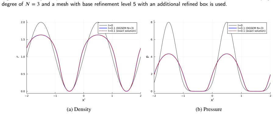
- Section 3.2: The isentropic flow test uses gamma=3, while the rest of the paper uses gamma=1.4. This should be stated more prominently, as it affects the near-vacuum conditions.
- Figure 9a: The y-axis label is unclear. Specifying that it shows the weighted average of limiting factors would help.
- Section 3.5: The domain is shortened to [0, 3.25] compared to the original [0, 4]. This should be noted as a deviation from the standard benchmark.
- Remark 8 discusses sensitivity of results to minor setup differences. While this is an honest disclosure, it would benefit from a more specific statement about which results are affected and to what degree.
- References: The self-citations [17, 18] are appropriate but frequent. The authors should ensure that the present contribution is clearly distinguished from [18], which also deals with monolithic convex limiting for LGL-DGSEM.
- No reproducible code or data is shipped with the paper ('Access to data and software is granted upon request'). For a methodological paper with extensive numerical experiments, providing a reproducibility artifact would strengthen the contribution.
Simulated Author's Rebuttal
We thank the referee for a careful and constructive report. The three major comments are well-taken, and we agree that the manuscript needs revisions to clarify the scope of the IDP guarantee and to label experiments more transparently. We address each comment below.
read point-by-point responses
-
Referee: Section 2.4: The solution transfer operators used during AMR refinement and coarsening are not invariant-domain-preserving, and the authors acknowledge this explicitly. The Zhang–Shu scaling limiter is a heuristic post-processing step, not a provable IDP mechanism. This means the overall scheme's IDP guarantee is broken at every refinement/coarsening event, regardless of the mortar flux correctness. Since AMR is a central feature of the paper's contribution, this gap is load-bearing for the claim of a unified IDP-AMR framework. The authors should either (a) clearly scope the IDP claim to the time-stepping update only, with the transfer step explicitly excluded from the guarantee, or (b) provide a more rigorous argument for why the Zhang–Shu limiter suffices.
Authors: The referee is correct on the substance. The solution transfer operators (interpolation for refinement, L2 projection for coarsening) are not IDP, and the Zhang–Shu scaling limiter we apply is a heuristic positivity-stabilizing post-processing step, not a provable mechanism for restoring admissibility in all cases. We do not have a rigorous argument that would elevate option (b) to a theorem, so we will adopt option (a). Specifically, we will revise the abstract, the introduction, and the conclusion to scope the IDP guarantee explicitly to the time-stepping update (i.e., the semi-discrete low-order scheme and the convex-limiting correction stage), and to state clearly that the solution transfer step is excluded from the IDP guarantee. Section 2.4 already contains the disclaimer ('We do not claim that this transfer operator is invariant-domain preserving in the strict sense'), but we will strengthen this language and add a forward reference from the abstract and conclusion so that the scope is unambiguous. We will also add a brief remark noting that constructing a provably IDP transfer operator for high-order DGSEM is an open problem and a target for future work. revision: yes
-
Referee: Remark 6 and Section 3.4: The IDP time-step restriction (44) is acknowledged to be more restrictive than the standard low-order CFL condition (47), and the authors describe a practical workaround that bypasses the bar-state bounds entirely, using low-order-solution-based bounds instead. This workaround is used in several numerical experiments (isentropic flow: CFL=0.5 with Eq. 47; KHI: CFL=0.2 with Eq. 47; Sedov with low-order bounds: CFL=0.4 with Eq. 47). When this workaround is used, the scheme is no longer provably IDP. The paper should clearly state in each experiment's description which CFL condition and which bound type are used, and should avoid presenting results obtained under the non-IDP workaround as validation of the IDP scheme. A table summarizing which experiments use the provably IDP configuration would help.
Authors: We agree. The distinction between the provably IDP configuration (bar-state bounds + CFL condition (44)) and the practical workaround (low-order-solution-based bounds + CFL condition (47)) is important and should be stated explicitly for each experiment. We will add a summary table (new Table) listing, for each numerical experiment: the bound type (bar-state local bounds, low-order-solution-based bounds, or positivity-only), the CFL condition used ((44) or (47)), the CFL number, and whether the configuration is provably IDP. We will also add a sentence at the beginning of each experiment's description cross-referencing this table. To be precise about the current state of the manuscript: the advection convergence test (Section 3.1) uses the IDP CFL condition (44) with CFL=0.95; the isentropic flow test (Section 3.2) uses the low-order CFL (47) with CFL=0.5 and positivity limiting (non-IDP workaround); the KHI (Section 3.3) uses CFL (47) with CFL=0.2 and positivity limiting (non-IDP workaround); the Sedov blast (Section 3.4) presents both configurations — bar-state bounds with CFL (44) at CFL=0.95 (provably IDP) and low-order-solution-based bounds with CFL (47) at CFL=0.4 (non-IDP workaround); the Double Mach reflection (Section 3.5) uses bar-state bounds with CFL (44) at CFL=0.9 (provably IDP); and the astrophysical jet (Section 3.6) uses bar-state bounds with CFL (44) at CFL=0.9 (provably IDP). We will make all of this explicit in the revised text and ensure that results obtained under the non-IDP workaround are not presented as validation of the IDP property, but rather as demonstrations of practical robustness. revision: yes
-
Referee: Section 2.3, Remark 7: The mortar limiting uses one limiting factor per mortar, and the admissible correction budget at a node is divided among all incident mortar contributions by scaling each anti-diffusive flux by n_i (the number of active mortar contributions). This is a conservative heuristic, but it is potentially suboptimal and may introduce more dissipation than necessary. The authors should discuss whether this division strategy preserves the formal accuracy of the high-order scheme in smooth regions (i.e., whether alpha_S -> 0 at the designed rate as the mesh is refined). The convergence results in Table 2 (local limiting, EOC ~ 1) suggest significant dissipation, but it is unclear how much of this is due to the mortar limiting strategy versus the local bounds themselves.
Authors: The referee raises a valid question about whether the n_i-scaling strategy preserves formal high-order accuracy in smooth regions. We do not have a formal proof that alpha_S -> 0 at the designed rate under mesh refinement when the n_i-scaling is used. However, we can offer the following observations. First, the EOC~1 result in Table 2 (local limiting with N=3) is consistent with what is observed in the conforming case with local limiting — see, e.g., [17, Table 4] where the conforming subcell limiting with local bounds also yields EOC~1. Since the conforming case has no mortar limiting at all, the reduced order of convergence is primarily attributable to the local bounds themselves (which enforce discrete maximum principles and thus introduce O(h) dissipation), not to the mortar limiting strategy per se. Second, the advection convergence test with positivity limiting only (Table 1) achieves full high-order convergence (EOC~4 for N=3), which shows that the mortar flux construction and the mortar limiting framework do not degrade accuracy when the local bounds are inactive. Third, the n_i-scaling is a conservative heuristic in the sense that it guarantees the sum of all mortar corrections stays within the admissible interval, but it is indeed potentially suboptimal. A tighter analysis could use a Zalesak-type synchronized limiting across all mortars incident on a node, but this would require a coupled solve and is significantly more complex to implement. We will add a remark to Section 2.3 discussing these points: (i) the EOC~1 is consistent with the conforming local-limiting case and is dominated by the local bounds, not the mortar strategy; (ii) the n_i-scaling is conservative but potentially suboptimal; and (iii) a synchronized Zalesak-type mortar limiter is a natural, revision: no
Circularity Check
No significant circularity found; the derivation is parameter-free and self-contained.
full rationale
The paper's central derivation chain is not circular. The sparse mortar fluxes (Eqs. 31-32) are constructed from local weights defined by LGL subcell characteristic functions (Eq. 26), which are geometric quantities determined by the subcell layout — not fitted to target data. Conservation (Eq. 25) follows from the symmetry of the weights and n_S^+ = -n_S^- (Eq. 24 vs. 21). The discrete metric identity (Eq. 38) extends to the nonconforming case because the partition of unity (Eq. 28) holds for characteristic functions by construction, yielding Eq. (39) = (1/2) ω_{i,S}^- n_S^- — the same value the volume SBP terms cancel. The bar-state form (Eq. 42) is a standard algebraic rearrangement of the low-order update (Eq. 11) using the metric identity, and the IDP property follows from the convexity of bar-states (Eq. 40) under the CFL restriction (Eq. 44), which is derived, not fitted. Self-citations [17, 18] provide the conforming-case foundation, but the nonconforming extension is independently derived: the sparsification (Eq. 26), the weight properties (Eq. 28), the metric identity extension (Eq. 39), and the IDP proof are all carried out in this paper. The conforming reduction (Eq. 33) is a consistency check, not a circular definition. The solution transfer gap (Section 2.4) is an acknowledged practical limitation, not a circularity in the mortar flux derivation. No step reduces to its inputs by construction or by unverified self-citation chain. Score 1 reflects minor self-citation to [17, 18] for the conforming-case framework, which is not load-bearing for the nonconforming extension's independent derivation.
Axiom & Free-Parameter Ledger
free parameters (3)
- beta (positivity lower bound scaling) =
0.1
- CFL number =
varies (0.2-0.95)
- global positivity threshold =
1e-10 or 1e-6
axioms (4)
- standard math The invariant domain G is convex and the bar-states lie in G if the nodal states do (convexity of LLF/HLL intermediate states).
- standard math SSP-RK methods can be written as convex combinations of forward Euler steps.
- domain assumption Nonconforming interfaces are 2-to-1 connections with same polynomial degree on both sides.
- ad hoc to paper The Zhang-Shu scaling limiter sufficiently stabilizes solution transfer during AMR.
Reference graph
Works this paper leans on
-
[1]
T. C. Fisher, M. H. Carpenter, High-order entropy stable finite difference schemes for nonlinear conservation laws: Finite domains, Journal of Computational Physics 252 (2013) 518–557
work page 2013
-
[2]
G. J. Gassner, A. R. Winters, D. A. Kopriva, Split form nodal discontinuous Galerkin schemes with summation-by-parts property for the compressible Euler equations, Journal of Computational Physics 327 (2016) 39–66
work page 2016
-
[3]
H.Ranocha,M.Schlottke-Lakemper,J.Chan,A.M.Rueda-Ramírez,A.R.Winters,F.Hindenlang,G.J.Gassner, Efficientimplementationof modernentropystableandkineticenergypreservingdiscontinuousGalerkinmethodsforconservationlaws, arXivpreprintarXiv:2112.10517 (2021)
work page internal anchor Pith review Pith/arXiv arXiv 2021
-
[4]
S. T. Zalesak, Fully multidimensional flux-corrected transport algorithms for fluids, Journal of Computational Physics 31 (1979) 335–362
work page 1979
-
[5]
Selmin, Finite element solution of hyperbolic equations
V. Selmin, Finite element solution of hyperbolic equations. II. Two-dimensional case, Research Report RR-0708, INRIA, 1987
work page 1987
- [6]
-
[7]
D.Kuzmin,R.Löhner,S.Turek(Eds.),Flux-CorrectedTransport:Principles,Algorithms,andApplications,2ed.,Springer,Dordrecht,2012
work page 2012
-
[8]
C.Lohmann,D.Kuzmin,J.N.Shadid,S.Mabuza, Flux-correctedtransportalgorithmsforcontinuousGalerkinmethodsbasedonhighorder Bernstein finite elements, Journal of Computational Physics 344 (2017) 151–186
work page 2017
-
[9]
R.Löhner,AppliedComputationalFluidDynamicsTechniques:AnIntroductionBasedonFiniteElementMethods,2ed.,JohnWiley&Sons, Chichester, 2008
work page 2008
- [10]
-
[11]
J. L. Guermond, B. Popov, Invariant domains and first-order continuous finite element approximation for hyperbolic systems, SIAM Journal on Numerical Analysis 54 (2016) 2466–2489
work page 2016
-
[12]
J.-L. Guermond, M. Nazarov, B. Popov, I. Tomas, Second-order invariant domain preserving approximation of the Euler equations using convex limiting, SIAM Journal on Scientific Computing 40 (2018) A3211–A3239
work page 2018
-
[13]
J.-L. Guermond, B. Popov, I. Tomas, Invariant domain preserving discretization-independent schemes and convex limiting for hyperbolic systems, Computer Methods in Applied Mechanics and Engineering 347 (2019) 143–175
work page 2019
-
[14]
W. Pazner, Sparse invariant domainpreserving discontinuous Galerkin methodswith subcell convex limiting, Computer Methods in Applied Mechanics and Engineering 382 (2021) 113876
work page 2021
-
[15]
H.Hajduk, MonolithicconvexlimitingindiscontinuousGalerkindiscretizationsofhyperbolicconservationlaws, Computers&Mathematics With Applications 87 (2021) 120–138. Bolm, Rueda-Ramírez, Kuzmin, Gassner:Preprint submitted to ElsevierPage 28 of 30 Invariant-domain-preserving mortar flux for LGL-DGSEM Node𝑗∈ + 𝑆 lower element upper element 0 1 2 3 4 0 1 2 3 4 N...
work page 2021
- [16]
-
[17]
A.M.Rueda-Ramírez,W.Pazner,G.J.Gassner, SubcelllimitingstrategiesfordiscontinuousGalerkinspectralelementmethods, Computers & Fluids 247 (2022) 105627
work page 2022
-
[18]
A. M. Rueda-Ramírez, B. Bolm, D. Kuzmin, G. J. Gassner, Monolithic convex limiting for legendre-gauss-lobatto discontinuous galerkin spectral-element methods, Communications on Applied Mathematics and Computation (2024)
work page 2024
-
[19]
D. A. Kopriva, A conservative staggered-grid chebyshev multidomain method for compressible flows. ii. a semi-structured method, Journal of Computational Physics 128 (1996) 475–488
work page 1996
-
[20]
H. Ranocha, M. Schlottke-Lakemper, A. R. Winters, E. Faulhaber, J. Chan, G. Gassner, Adaptive numerical simulations with Trixi.jl: A case study of Julia for scientific computing, Proceedings of the JuliaCon Conferences 1 (2022) 77
work page 2022
- [21]
-
[22]
D.Kuzmin, Entropystabilizationandproperty-preservinglimitersfordiscontinuousGalerkindiscretizationsofnonlinearhyperbolicequations (2020)
work page 2020
-
[23]
R. Anderson, V. Dobrev, T. Kolev, D. Kuzmin, M. Quezada de Luna, R. Rieben, V. Tomov, High-order local maximum principle preserving (MPP) discontinuous Galerkin finite element method for the transport equation, Journal of Computational Physics 334 (2017) 102–124
work page 2017
-
[24]
D.Kuzmin,M.QuezadadeLuna, Subcellfluxlimitingforhigh-orderBernsteinfiniteelementdiscretizationsofscalarhyperbolicconservation laws, Journal of Computational Physics 411 (2020) 109411
work page 2020
-
[25]
S. Hennemann, A. M. Rueda-Ramírez, F. J. Hindenlang, G. J. Gassner, A provably entropy stable subcell shock capturing approach for high order split form DG for the compressible Euler equations, Journal of Computational Physics 426 (2021) 109935
work page 2021
-
[26]
part ii: Subcell finite volume shock capturing, Journal of Computational Physics 444 (2021) 110580
A.M.Rueda-Ramírez,S.Hennemann,F.J.Hindenlang,A.R.Winters,G.J.Gassner, AnentropystablenodaldiscontinuousGalerkinmethod for the resistive mhd equations. part ii: Subcell finite volume shock capturing, Journal of Computational Physics 444 (2021) 110580
work page 2021
-
[27]
A.M.Rueda-Ramírez,G.J.Gassner, Asubcellfinitevolumepositivity-preservinglimiterforDGSEMdiscretizationsoftheEulerequations, arXiv preprint2102.06017 [math.NA](2021)
work page internal anchor Pith review Pith/arXiv arXiv 2021
- [28]
-
[29]
D. Kuzmin, H. Hajduk, A. Rupp, Limiter-based entropy stabilization of semi-discrete and fully discrete schemes for nonlinear hyperbolic problems, Computer Methods in Applied Mechanics and Engineering 389 (2022) 114428. Bolm, Rueda-Ramírez, Kuzmin, Gassner:Preprint submitted to ElsevierPage 29 of 30 Invariant-domain-preserving mortar flux for LGL-DGSEM
work page 2022
-
[30]
X. Zhang, C.-W. Shu, Maximum-principle-satisfying and positivity-preserving high-order schemes for conservation laws: Survey and new developments, Proceedings of the Royal Society A: Mathematical Physical and Engineering Sciences 467 (2011) 2752–2776
work page 2011
-
[31]
H.Ranocha,GeneralisedSummation-by-PartsOperatorsandEntropyStabilityofNumericalMethodsforHyperbolicBalanceLaws,Cuvillier Verlag, Göttingen, 2018
work page 2018
-
[32]
C.-W. Shu, S. Osher, Efficient implementation of essentially non-oscillatory shock-capturing schemes, Journal of Computational Physics 77 (1988) 439–471
work page 1988
-
[33]
C.Burstedde,L.C.Wilcox,O.Ghattas,p4est:Scalablealgorithmsforparalleladaptivemeshrefinementonforestsofoctrees, SIAMJournal on Scientific Computing 33 (2011) 1103–1133
work page 2011
-
[34]
J. Cheng, C.-W. Shu, Positivity-preserving lagrangian scheme for multi-material compressible flow, Journal of Computational Physics 257 (2014) 143–168
work page 2014
-
[35]
F. Vilar, A posteriori correction of high-order discontinuous Galerkin scheme through subcell finite volume formulation and flux reconstruction, Journal of Computational Physics 387 (2019) 245–279
work page 2019
-
[36]
P. Bacigaluppi, R. Abgrall, S. Tokareva, “a posteriori” limited high order and robust schemes for transient simulations of fluid flows in gas dynamics, Journal of Computational Physics 476 (2023) 111898
work page 2023
-
[37]
R. Löhner, An adaptive finite element scheme for transient problems in cfd, Computer Methods in Applied Mechanics and Engineering 61 (1987) 323–338
work page 1987
-
[38]
B. Fryxell, K. Olson, P. Ricker, F. Timmes, M. Zingale, D. Lamb, P. MacNeice, R. Rosner, J. Truran, H. Tufo, Flash: An adaptive mesh hydrodynamics code for modeling astrophysical thermonuclear flashes, The Astrophysical Journal Supplement Series 131 (2000) 273
work page 2000
-
[39]
A. M. Rueda-Ramírez, G. J. Gassner, A flux-differencing formula for split-form summation by parts discretizations of non-conservative systems: Applications to subcell limiting for magneto-hydrodynamics, arXiv preprint arXiv:2211.14009 (2022)
work page internal anchor Pith review Pith/arXiv arXiv 2022
-
[40]
P. Woodward, P. Colella, The numerical simulation of two-dimensional fluid flow with strong shocks, Journal of Computational Physics 54 (1984) 115–173
work page 1984
-
[41]
D. Kuzmin, Monolithic convex limiting for continuous finite element discretizations of hyperbolic conservation laws, Computer Methods in Applied Mechanics and Engineering 361 (2020) 112804
work page 2020
-
[42]
Y. Ha, C. L. Gardner, A. Gelb, C.-W. Shu, Numerical simulation of high mach number astrophysical jets with radiative cooling, Journal of Scientific Computing 24 (2005) 29–44
work page 2005
-
[43]
P. Chandrashekar, Kinetic energy preserving and entropy stable finite volume schemes for compressible Euler and Navier–Stokes equations, Communications in Computational Physics 14 (2013) 1252–1286
work page 2013
-
[44]
Bolm, Rueda-Ramírez, Kuzmin, Gassner:Preprint submitted to ElsevierPage 30 of 30
N.Fleischmann,S.Adami,N.A.Adams,Numericalsymmetry-preservingtechniquesforlow-dissipationshock-capturingschemes,Computers & Fluids 189 (2019) 94–107. Bolm, Rueda-Ramírez, Kuzmin, Gassner:Preprint submitted to ElsevierPage 30 of 30
work page 2019
discussion (0)
Sign in with ORCID, Apple, or X to comment. Anyone can read and Pith papers without signing in.