pith. sign in

arxiv: 2606.02711 · v1 · pith:FDVMUEC5new · submitted 2026-06-01 · 🌌 astro-ph.GA · astro-ph.CO

Lyman-alpha Pressure Strongly Enhances Pre-Supernova Feedback at Cosmic Dawn: The First Multi-Dimensional Lyman-alpha Radiation Hydrodynamics Simulations

Pith reviewed 2026-06-28 13:33 UTC · model grok-4.3

classification 🌌 astro-ph.GA astro-ph.CO
keywords Lyman-alpharadiation pressurefeedbackcosmic dawnradiation hydrodynamicsmetal-pooroutflowsstar formation
0
0 comments X

The pith

Lyα radiation pressure dominates pre-supernova feedback by factors of 10-60 in dense metal-poor clouds at cosmic dawn.

A machine-rendered reading of the paper's core claim, the machinery that carries it, and where it could break.

The paper runs the first two-dimensional radiation hydrodynamics simulations that include Lyman-alpha transfer for star clusters and isolated stars inside dense, metal-poor gas. It shows that Lyα photons create strong radiation pressure inside H II regions even when some photons leak through low-column channels or shift in frequency. This pressure produces forces several times larger than the star's total luminosity divided by the speed of light and drives much stronger outflows than direct starlight or infrared radiation can achieve. The work concludes that nearly every existing galaxy and star-formation simulation omits the main radiation-pressure channel operating at cosmic dawn.

Core claim

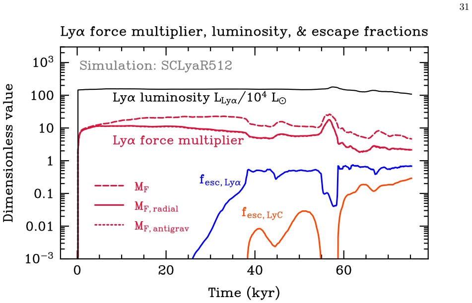
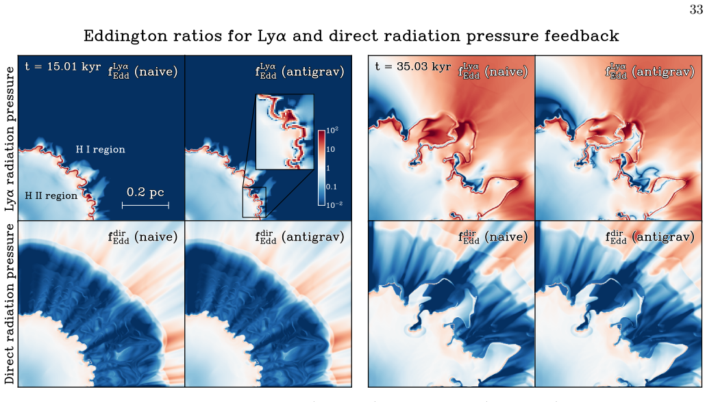
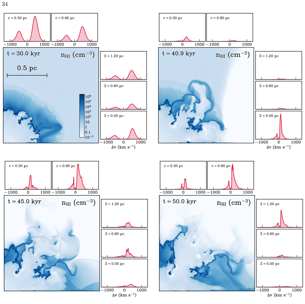
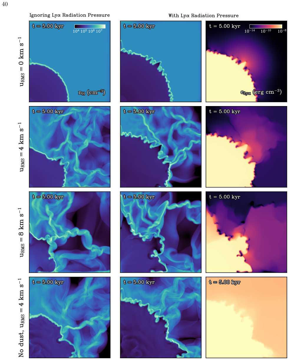
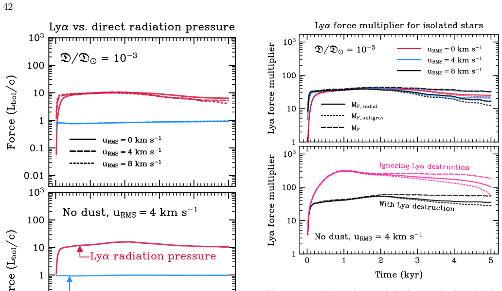
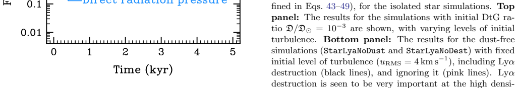
Using the Lydion code, the simulations demonstrate that Lyman-alpha radiation pressure generates radiative forces of (2-16) times L_bol/c with force multipliers of 10-60 in metal-poor environments, dominating over other radiation pressures and enhancing outflows, although Lyα leakage through channels, Doppler shifts, and photon destruction cannot prevent the build-up of strong pressure in H II regions.

What carries the argument

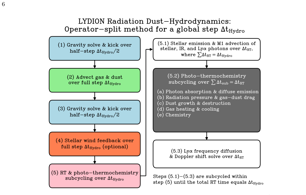
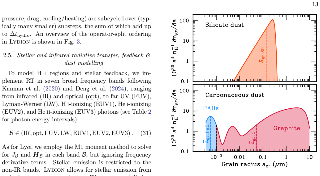
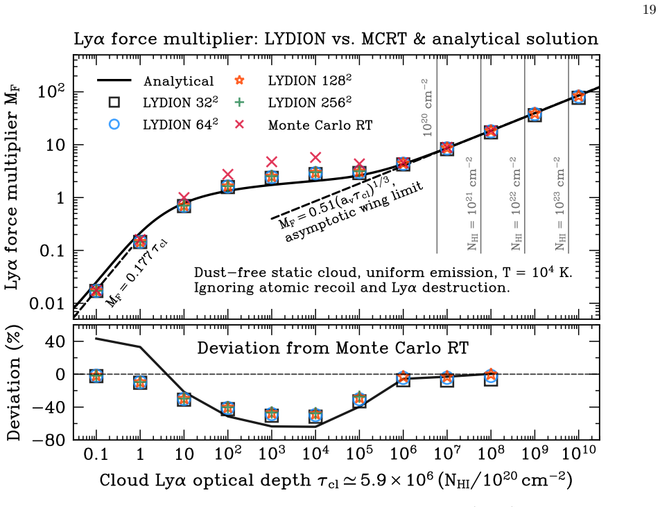
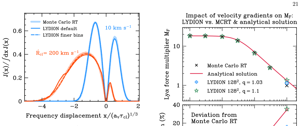
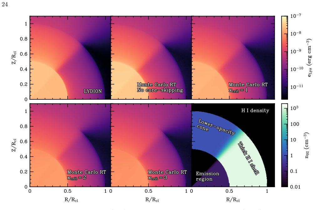
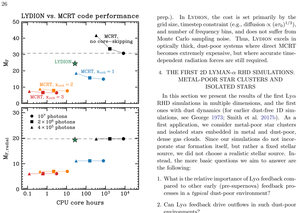
Lydion, an RHD code that uses a novel M1 moment closure for Lyman-alpha radiative transfer together with self-consistent dust dynamics, allowing multi-dimensional runs at roughly one-hundred times the speed of Monte Carlo methods.

If this is right

  • Lyα feedback dramatically boosts outflows in the pre-supernova phase of star formation.
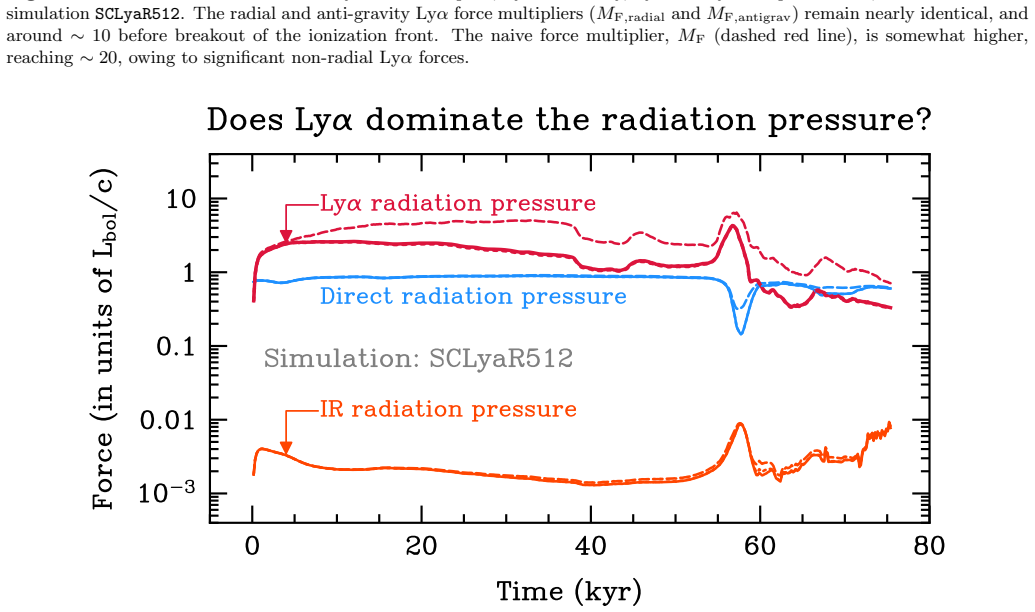
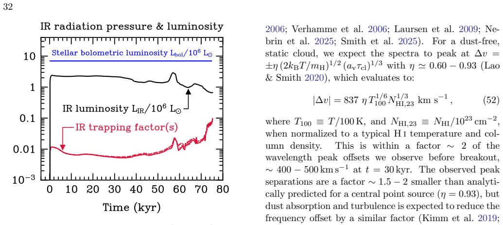
  • It produces radiative forces several times larger than those from direct stellar or infrared radiation pressure.
  • Nearly all current galaxy and star-formation simulations miss the strongest source of radiation pressure in dense, metal-poor gas.
  • Efficient star formation requires a higher gas surface density than models without Lyα pressure predict.
  • Lyα leakage and destruction do not eliminate the strong pressure build-up inside H II regions.

Where Pith is reading between the lines

These are editorial extensions of the paper, not claims the author makes directly.

  • The enhanced feedback could lower the escape fraction of ionizing photons from the first galaxies.
  • High-redshift observations of fast galactic outflows might be compared against the predicted force-multiplier range.
  • Adding the effect to cosmological simulations would shift the timing and efficiency of star formation at cosmic dawn.
  • Three-dimensional versions of the simulations could reveal how asymmetric gas geometries change the reported multipliers.

Load-bearing premise

The M1 moment closure for Lyα radiative transfer remains accurate enough in multi-dimensional H II regions with Doppler shifts, leakage channels, and dust to produce reliable force multipliers.

What would settle it

A side-by-side 2D simulation of the same star-cluster setup run once with the M1 method and once with full Monte Carlo Lyman-alpha transfer, checking whether the force multipliers and outflow velocities agree within the reported range.

Figures

Figures reproduced from arXiv: 2606.02711 by Aaron Smith, Daniele Manzoni, Garrelt Mellema, Kevin Lorinc, Olof Nebrin.

Figure 1
Figure 1. Figure 1: Simulations of a compact (Rh = 0.05 pc), low-mass (104 M⊙) star cluster in an initially dense (nH = 105 cm−3 ), dust-poor (D/D⊙ = 0.01) cloud, with (right panels) and without (left panels) Lyα radiation pressure feedback. Plots show the gas density nH, and, for the run with Lyα RT, the Lyα energy density eLyα. Also shown are forces from Lyα, direct, and IR radiation pressure, as well as the Lyα escape frac… view at source ↗
Figure 2
Figure 2. Figure 2: Same as [PITH_FULL_IMAGE:figures/full_fig_p004_2.png] view at source ↗
Figure 3
Figure 3. Figure 3: A schematic overview of the operator-split method used in Lydion to advance gas, dust, radiation (including Lyα), and thermochemistry over each global time-step ∆tHydro. Each step is described in more detail in the main text and Appendices, although not necessarily in the order they are updated in a simulation time-step (the actual order used is shown in this figure). Nebrin et al. 2025; Smith et al. 2025)… view at source ↗
Figure 4
Figure 4. Figure 4: The default Lyα frequency grid adopted in Lydion, along with the Voigt profile for two representative temperatures, T = 100 K and T = 104 K. Dashed lines show the frequency bin interfaces, highlighting that the core of the line is always resolved. Note that the full frequency grid is not shown here, which extends to |ν − νLyα| = 105 ∆νD(30 K). limiter.10 We adopt the Global Lax-Friedrichs (GLF) approximate… view at source ↗
Figure 5
Figure 5. Figure 5: The Lyα emission probability PLyα per recombi￾nation event as a function of temperature and electron den￾sity for Case A (top panel) and Case B recombinations (bot￾tom panel), as computed by Storey & Hummer (1995). Here ELyα ≃ 10.2 eV is the Lyα photon energy, PLyα is the probability that a recombination event will pro￾duce a Lyα photon, krec(T) is the recombination co￾efficient, kcoll(T) the collisional e… view at source ↗
Figure 6
Figure 6. Figure 6: The dust grain size distribution for silicate grains (top panel) and carbonaceous grains (bottom panel) for the RV = 5.5, bC = 3 × 10⁻⁵ , case B dust model of Weingartner & Draine (2001a), for their fiducial Milky Way dust abundance (cf. their fig. 6). We split up the latter into PAHs (< 10−3 µm) and graphite dust (> 10−3 µm). We have also marked the area-weighted mean grain sizes, a¯gr ≡ ⟨a 3 gr⟩/⟨a 2 gr⟩… view at source ↗
Figure 7
Figure 7. Figure 7: The predicted force multiplier MF for clouds of varying Lyα optical depth τcl (Test 1). Lydion predictions for different spatial resolutions 322−2562 are shown (symbols), together with analytical predictions (solid line, using the closed-form solution of Tomaselli & Ferrara 2021), and MCRT results from colt (diamonds) for 0.1 ≤ τcl ≤ 108 . In the top panel, dashed black lines show the asymptotic relations … view at source ↗
Figure 8
Figure 8. Figure 8: Predicted normalized emergent spectra from static dust-free clouds, of temperature T = 104 K, with uniform Lyα emission, and ignoring atomic recoil (Test 1). Dashed lines show the analytical solution of Lao & Smith (2020). Solid lines show the spectra obtained from Ly￾dion (for spatial resolution 1282 ), at the outer R and Z￾boundaries. 0 0.2 0.4 0.6 0.8 1 Spherical radius r/Rcl 0 1 2 3 4 5 6 e L y ( 1 0 8… view at source ↗
Figure 9
Figure 9. Figure 9: The predicted spherically averaged Lyα energy density profile eLyα(r), for the dust-free static cloud setup (Test 1: τcl = 1010 , T = 104 K, uniform Lyα emission, ig￾noring atomic recoil). Solid lines show the Lydion results (for spatial resolution 1282 ) at different times t, in units of tdiff ≡ (avτcl) 1/3Rcl/c. The dashed pink line shows the an￾alytical solution of Lao & Smith (2020) for the same setup.… view at source ↗
Figure 10
Figure 10. Figure 10: Emergent spectra (averaged over all boundary cells), for expanding dust-free uniform clouds of optical depth τcl = 5 × 10⁸ , temperature T = 9084 K, and uniform Lyα emission (Test 2). Solid and dashed lines show spectra from Lydion with the default and higher number of frequency bins, respectively. Bands show MCRT results from Smith et al. (2025). just note that discrepancies with respect to MCRT only app… view at source ↗
Figure 11
Figure 11. Figure 11: Suppression of the Lyα force multiplier MF with increasing cloud expansion rates R˙ cl, for a uniform dust￾free cloud with temperature T = 104 K, Lyα optical depth τcl = 108 at line center, and uniform Lyα emission (Test 2). Atomic recoil is ignored. Top panel: Lydion predictions are shown as symbols for a fixed spatial resolution of 1282 . We run one simulation with more frequency bins (q = 1.03) for the… view at source ↗
Figure 13
Figure 13. Figure 13: The Lyα escape fraction for different cloud con￾tinuum absorption optical depths τc, and for different source distributions (Test 4): uniform Lyα emission (gray), and central point-like emission (red). Symbols show results from Lydion for a few values of τc, and for different spatial resolu￾tions (322 − 1282 , plus one simulation at 2562 ). Bands show MCRT results from colt assuming a modest static core￾s… view at source ↗
Figure 14
Figure 14. Figure 14: Suppression of the Lyα force multiplier MF with increasing dust absorption optical depth τc, for a uniform cloud with temperature T = 104 K, Lyα optical depth τcl = 108 at line center, and uniform Lyα emission (Test 5). Top panel: Lydion predictions are shown as symbols for varying spatial resolution, 322 − 2562 . MCRT results from colt are shown as crosses. The analytical solution of Nebrin et al. (2025)… view at source ↗
Figure 15
Figure 15. Figure 15: The Lyα energy density eLyα(R, Z) and H i density for the anisotropic cone test (Test 6). Top left panel: The predicted eLyα from Lydion. Top middle and right panels: The predicted eLyα from colt, without core-skipping (middle panel), and with modest core-skipping (right panel, xcrit = 1). Bottom left and middle panels: The predicted eLyα from colt, with increasing levels of core-skipping. Bottom right pa… view at source ↗
Figure 16
Figure 16. Figure 16: Same as [PITH_FULL_IMAGE:figures/full_fig_p025_16.png] view at source ↗
Figure 18
Figure 18. Figure 18: CPU core hours for the anisotropic cone test run on a MacBook Pro laptop (Apple M2 chip with 16 GB RAM) using 8 CPU threads, for varying spatial resolutions 322 –2562 . The final time, tmax = 4 tdiff , and the number of frequency bins are fixed. The dashed line shows the expected N 3 scaling for a spatial resolution of N 2 [PITH_FULL_IMAGE:figures/full_fig_p025_18.png] view at source ↗
Figure 19
Figure 19. Figure 19: The naive and radial force multipliers MF (top panel) and MF,radial (bottom panel), respectively, for the anisotropic cone test. The results are plotted against the CPU core hours, as reported in Lydion and all the MCRT calculations. For the latter, we show results with and without core-skipping, and varying number of photons (4 × 10⁵ − 107 ). The dashed gray lines highlight the force multipliers for the … view at source ↗
Figure 20
Figure 20. Figure 20: In this plot we show the assumed initial DtG ratios and gas metallicities for the subset of Lydion runs with dust, and how they compare to various low and high-redshift objects. We show low-redshift trends for galaxies from R´emy-Ruyer et al. (2014), and Galliano et al. (2021) (black dashed, and orange solid line, respectively). Gray squares show quasar absorbers at redshift z ∼ 0 − 5 from P´eroux & Howk … view at source ↗
Figure 21
Figure 21. Figure 21: The evolution of the potentially star-forming gas mass (top panel), and total gas mass remaining in the simulation volume (bottom panel), for the star cluster simu￾lations. Solid (dashed) lines show the results when incorpo￾rating (ignoring) Lyα pressure. Lyα feedback is expected to suppress star formation for this particular setup. rently modelled in Lydion, we can estimate the mass of dense gas that wou… view at source ↗
Figure 22
Figure 22. Figure 22: Plot of the evolution of the Lyα force multiplier, Lyα luminosity, Lyα and LyC escape fractions, for the star cluster simulation SCLyaR512. The radial and anti-gravity Lyα force multipliers (MF,radial and MF,antigrav) remain nearly identical, and around ∼ 10 before breakout of the ionization front. The naive force multiplier, MF (dashed red line), is somewhat higher, reaching ∼ 20, owing to significant no… view at source ↗
Figure 23
Figure 23. Figure 23: Comparison of forces from Lyα, direct, and IR radiation pressure, for the star cluster simulation SCLyaR512. Naive, radially outward, and antigravity forces are shown as dashed, solid, and dotted lines, respectively. Radial and antigravity forces largely overlap, whereas naive and radial forces can differ significantly for Lyα pressure [PITH_FULL_IMAGE:figures/full_fig_p031_23.png] view at source ↗
Figure 24
Figure 24. Figure 24: Plot of the IR luminosity (black line), stel￾lar bolometric luminosity (blue line), and IR radiation force trapping factors (red lines). The latter are shown for the naive, radial, and antigravity forces (c.f [PITH_FULL_IMAGE:figures/full_fig_p032_24.png] view at source ↗
Figure 25
Figure 25. Figure 25: Maps from SCLyaR512, at t = 15 kyr (left panels) and t = 35 kyr (right panels), of the Eddington ratio fEdd ∼ (Radiation pressure force)/(Gravitational force) for both Lyα radiation pressure (top row), and direct (non-IR) ra￾diation pressure (bottom row). The Lyα radiation pressure force is highly concentrated near the shock/ionization front, with extreme Eddington ratios reaching few × 10 ≲ f Lyα Edd ≲ 1… view at source ↗
Figure 26
Figure 26. Figure 26: Lyα emergent spectra before (t = 30 kyr) and after (t ≳ 41 kyr) breakout of the ionization front in the simulation SCLyaR512. Color maps show the H i number density for the full 1.2 pc×1.2 pc box, with dark regions highlighting dense H i gas. Emergent Lyα spectra, taken near simulation box boundaries, are shown above (for the upper Z-boundary) and to the right (for the outer R-boundary) of the respective … view at source ↗
Figure 27
Figure 27. Figure 27: Dust properties (and the gas temperature for comparison) roughly at t = 15 kyr in the high-resolution Lyα RHD simulation (SCLyaR512). Panel (a): The gas temperature. Panel (b): The total dust-to-gas ratio in Solar units. Panel (c): The fraction of dust mass in PAHs. Panel (d): The Lyα dust absorption cross-section per H nucleus (in cm2 H −1 ). Panels (e)–(f): The dust-to-gas ratios of silicate (Sil) and g… view at source ↗
Figure 28
Figure 28. Figure 28: Gas abundances (and the gas temperature for comparison) at t = 15 kyr in the high-resolution Lyα RHD simulation (SCLyaR512). Panel (a): The gas temperature. Panel (b): The H i abundance xHI ≡ nHI/nH. Panel (c): The H2 abundance xH2 ≡ nH2 /nH. Panel (d): The He i abundance xHeI ≡ nHeI/nHe. Panels (e): The He ii abundance xHeII ≡ nHeII/nHe. Panel (f): The He iii abundance xHeIII ≡ nHeIII/nHe. Panel (g): The… view at source ↗
Figure 29
Figure 29. Figure 29: The Lyα destruction probability pd at t = 15 kyr in the Lyα RHD simulation SCLyaR512. The destruction probability is ∼ 10−9 in the H ii region, and drops to ∼ 10−13 − 10−11 in the neutral gas. whether our results are converged.44 To check this, in [PITH_FULL_IMAGE:figures/full_fig_p037_29.png] view at source ↗
Figure 30
Figure 30. Figure 30: The evolution of various quantities (e.g. force multipliers), for all spatial resolutions (1282 − 5122 ) in the star cluster simulations. Top left panel: The net radial Lyα force multiplier MF,radial for the Lyα RHD simulations. Top right panel: The net Lyα force multiplier MF,antigrav in the opposite direction of gravity, for the Lyα RHD simulations. Middle left panel: The Lyα escape fraction. We note th… view at source ↗
Figure 31
Figure 31. Figure 31: The gas density and Lyα energy density eLyα for the simulations of the isolated stars of mass 35 M⊙, at t = 5 kyr, for different levels of initial turbulent velocities uRMS = 0 − 8 km s−1 . Each panel is 0.1 pc × 0.1 pc. The bottom row shows the results for the dust-free simulations (StarNoLyaNoDust, StarLyaNoDust), whereas the rest of the rows assume an initial DtG ratio of D/D⊙ = 10−3 . Lyα feedback is … view at source ↗
Figure 32
Figure 32. Figure 32: Same as [PITH_FULL_IMAGE:figures/full_fig_p041_32.png] view at source ↗
Figure 34
Figure 34. Figure 34: The evolution of the force multipliers (as de￾fined in Eqs. 43–49), for the isolated star simulations. Top panel: The results for the simulations with initial DtG ra￾tio D/D⊙ = 10−3 are shown, with varying levels of initial turbulence. Bottom panel: The results for the dust-free simulations (StarLyaNoDust and StarLyaNoDest) with fixed initial level of turbulence (uRMS = 4 km s−1 ), including Lyα destructi… view at source ↗
Figure 33
Figure 33. Figure 33: A comparison between Lyα and direct radia￾tion pressure forces for the isolated star simulations (similar to [PITH_FULL_IMAGE:figures/full_fig_p042_33.png] view at source ↗
Figure 35
Figure 35. Figure 35: Snapshots from the Sedov–Taylor blast wave test, for two resolutions: 1282 (a) and 5122 (b). In each panel, the dashed white line shows the expected spherically symmetric blast wave radius from the Sedov-Taylor solution, RST = 1.15167 (Eblastt 2 /ρ0) 1/5 (e.g. Ostriker & McKee 1988). 0.0 0.5 1.0 1.5 Radial distance 0 1 2 3 4 t = 0.400 Spherically averaged density LYDION 512 2 Analytical 0.0 0.5 1.0 1.5 Ra… view at source ↗
Figure 36
Figure 36. Figure 36: The spherically averaged density (left) and pressure (right) profiles at t = 0.4, for the Sedov-Taylor test at 5122 resolution (solid lines). Dashed lines show the analytical solution for comparison. value computed, and derive the corresponding cell-central values of all conservative variables using this τ . Furthermore, we also revert to τ = 1 if the corresponding pressure or density is still unphysical,… view at source ↗
Figure 37
Figure 37. Figure 37: Results for the Sod shock tube test at t = 0.2 for different resolutions. The numerical results for ρ (upper left panel), P (upper right panel), uX (lower left panel), and P/ρ (proxy for temperature, lower right panel), along with the exact analytical solution (dashed lines) are shown. B.2.1. Sedov-Taylor blast wave To test the ability of Lydion to handle strong shocks and to maintain reasonable symmetry,… view at source ↗
Figure 38
Figure 38. Figure 38: Four snapshots of the density ρ from the Rayleigh-Taylor instability test, for a resolution 256 × 768. B.2.3. Rayleigh-Taylor instability Next, we perform a Rayleigh-Taylor instability (RTI) test in a 2D Cartesian setup, of box length (Xmax, Ymax) = (0.5, 1.5).50 A uniform, time-independent gravitational field −∇Φ = −0.1 Yˆ is set up, with periodic and reflective boundary conditions in the X and Y directi… view at source ↗
Figure 39
Figure 39. Figure 39: Four snapshots of the gas density from the Kelvin-Helmholtz instability test, at a resolution of 5122 . method. Instead, we adopt a Peaceman-Rachford ADI method (Peaceman & Rachford 1955), wherein one treats one direction implicitly at a time. For a detailed description of the method applied to the Poisson equation, we refer the reader to Black & Bodenheimer (1975), Norman & Winkler (1986), and Stone & No… view at source ↗
Figure 40
Figure 40. Figure 40: Snapshots of the spherically averaged density profile for the nearly pressure-free collapse test, for two resolutions: NR = 128 (a) and NZ = 512 (b). In each panel, the dashed lines show the exact analytical solution for the density profile, for a pressure-free collapse (see eqs. 89–90 in Stone & Norman 1992). Solid lines show the numerical results without assumed mirror symmetry (NZ = 2NR), while dotted … view at source ↗
Figure 41
Figure 41. Figure 41: Results for the hydrostatic equilibrium test. Panel (a) shows the gas density at the final time t = 50 tdyn. Panel (b) shows the evolution of the spherically averaged density profile, compared to the analytical prediction from Eq. (C29). density outside the cloud is set to 10−5 ρc. If the implementation of gravity and hydrodynamics is accurate, then the cloud should maintain the equilibrium profile in Eq.… view at source ↗
Figure 42
Figure 42. Figure 42: D-type photoionization test. Left: Evolution of the ionization front radius (in units of the Str¨omgren radius) and velocity compared to the Capreole + C2 -ray reference solution. Right: Predicted H i fraction, gas pressure, temperature, and density profiles. Solid, short-dashed, and long-dashed lines show results from Lydion, Arepo-rt, and Capreole + C2 -ray, respectively. The profile comparison is shown… view at source ↗
Figure 43
Figure 43. Figure 43: Planck and Rosseland-mean dust opacities, as a function of temperature. Left panel: Opacities in a given dust bin (cm2 per gram of dust mass in that bin). Right panel: The total opacities (cm2 per gram of total dust mass), assuming the initial mass distribution for the RV = 5.5 dust model of Weingartner & Draine (2001a). The opacities scale approximately as ∝ T 2 for T ≲ 200 K, and then reach a plataeu ar… view at source ↗
Figure 44
Figure 44. Figure 44: The band-averaged photodetachment cross-sections, σH−,B ≡ [ R B dν Bν(Teff )σH− (ν)/hν]/[ R B dν Bν(Teff )/hν], as￾suming black-body spectra for (nearly) zero-metallicity stars (solid lines), and for metal-poor Z⋆/Z⊙ = 0.01 stars (dashed lines). Data for the cross-section is taken from McLaughlin et al. (2017), and Teff derived from the fits in Tanikawa et al. (2020). Note that the cross-section for the L… view at source ↗
Figure 45
Figure 45. Figure 45: The band-averaged O i and C i photoionization cross-sections for metal-poor Z⋆/Z⊙ = 0.01 stars. Fits for the cross-section were taken from Verner et al. (1996), and effective temperatures Teff were derived from the fits in Tanikawa et al. (2020). with COHx→CO = kOHx,CInOx n CI, with xCI/CII ≡ (nCI/CII)/nC (here and below). Next, we use the predictor values of (O i, O ii) to feed into an update of the carb… view at source ↗
Figure 46
Figure 46. Figure 46: The band-averaged OH, CH, and CO photodissociation cross-sections for metal-poor Z⋆/Z⊙ = 0.01 stars. Data for the cross-section were taken from Heays et al. (2017), and effective temperatures Teff were derived from the fits in Tanikawa et al. (2020). rates for these processes are therefore: Γ OI ion = 4π  JEUV1σOI,EUV1 EEUV1 + JEUV2σOI,EUV2 EEUV2 + JEUV3σOI,EUV3 EEUV3  , (G120) Γ CI ion = 4π  JLWσCI,LW… view at source ↗
read the original abstract

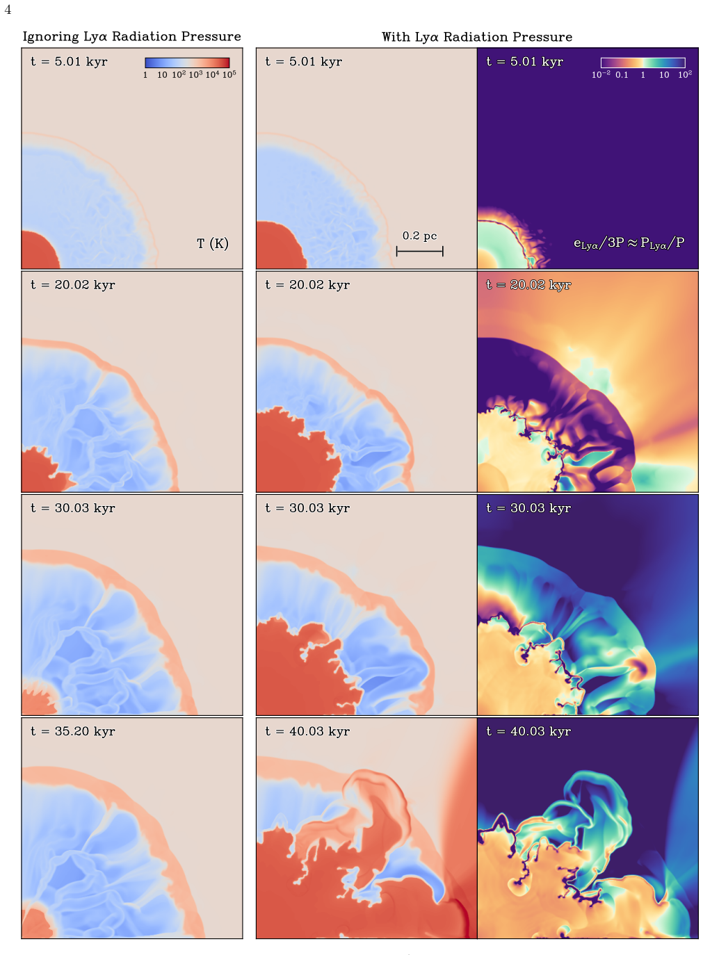
The dynamical role of Lyman-$\alpha$ (Ly$\alpha$) radiation pressure feedback has been debated for nearly a century, with recent analytical and 1D numerical studies highlighting its potential dominance over other stellar feedback processes at Cosmic Dawn. Despite this, no multi-dimensional Ly$\alpha$ radiation hydrodynamics (RHD) simulations have been performed to date. In this paper, we present the first 2D Ly$\alpha$ RHD simulations using Lydion, an RHD code with a novel M1 moment method for Ly$\alpha$ transfer, and self-consistent dust dynamics. Lydion yields a $\sim \mathcal{O}(100) \,\times$ speed-up compared to Monte Carlo radiative transfer in simple benchmarks, making 2D Ly$\alpha$ RHD feasible. We perform simulations of star clusters and isolated stars embedded in dense, metal-poor ($Z/Z_\odot \leq 0.01$) clouds, and find that Ly$\alpha$ feedback dramatically boosts outflows and dominates over feedback from direct and infrared radiation pressure. Ly$\alpha$ leakage through lower-column density channels, Doppler shifts, and Ly$\alpha$ photon destruction, while important, cannot prevent the build-up of strong Ly$\alpha$ radiation pressure in H II regions, leading to radiative forces $\sim (2 - 16) \times L_{\rm bol}/c$, and Ly$\alpha$ force multipliers $M_{\rm F} \sim 10-60$. Ly$\alpha$ feedback may not preclude efficient star formation, but raises the threshold gas surface density for this to occur. We conclude that nearly all galaxy and star formation simulations are currently missing the strongest source of radiation pressure feedback in dense and metal-poor environments.

Editorial analysis

A structured set of objections, weighed in public.

Desk editor's note, referee report, simulated authors' rebuttal, and a circularity audit. Tearing a paper down is the easy half of reading it; the pith above is the substance, this is the friction.

Referee Report

3 major / 2 minor

Summary. The paper presents the first 2D Lyman-alpha radiation hydrodynamics simulations using the Lydion code with a novel M1 moment closure for Lyα transfer and self-consistent dust dynamics. It simulates star clusters and isolated stars in dense, metal-poor (Z/Z⊙ ≤ 0.01) clouds and claims that Lyα feedback dramatically boosts outflows, dominates over direct and infrared radiation pressure, and produces radiative forces ∼(2-16)×L_bol/c with force multipliers M_F ∼10-60, even with leakage channels, Doppler shifts, and photon destruction; this implies Lyα is the strongest radiation pressure source at cosmic dawn and raises the gas surface density threshold for efficient star formation.

Significance. If the results hold, the work would identify a dominant pre-supernova feedback channel missing from nearly all current galaxy and star formation simulations in dense, low-metallicity regimes. The O(100)× speedup of the M1 solver relative to Monte Carlo on benchmarks is a technical strength that enables the multi-dimensional runs.

major comments (3)
  1. [§2 (Lydion M1 solver description)] §2 (Lydion M1 solver description): the M1 closure is applied to 2D H II regions with self-consistent velocity fields, leakage channels, and dust that generate the headline force multipliers, yet validation against Monte Carlo is reported only for simple benchmarks; no cross-check is shown for the anisotropic, Doppler-shifted geometries that produce M_F ∼10-60. This is load-bearing because the closure assumes a specific angular distribution whose failure would directly alter trapped photon density and net momentum deposition.
  2. [Results section reporting the (2-16)×L_bol/c and M_F ∼10-60 ranges] Results section reporting the (2-16)×L_bol/c and M_F ∼10-60 ranges: these quantitative values, which underpin the dominance claim over direct/IR pressure, are presented without resolution convergence tests, Monte Carlo cross-checks in the target setups, or error bars, as noted by the absence of such tests in the abstract and results.
  3. [Discussion/conclusions] Discussion/conclusions: the statement that leakage, Doppler shifts, and destruction cannot prevent strong Lyα pressure build-up rests entirely on the M1-derived radiation fields; without demonstrated accuracy of the closure in the simulated regimes, the conclusion that Lyα feedback raises the star-formation threshold cannot be separated from possible numerical artifacts.
minor comments (2)
  1. [Abstract] Abstract: the reported force and multiplier ranges are stated without reference to the number of runs, exact parameter variations, or which setups produce the extremes of the 2-16 and 10-60 intervals.
  2. [Notation] Notation: the definition of the force multiplier M_F should be given explicitly with an equation number on first use in the main text rather than only in a methods appendix.

Simulated Author's Rebuttal

3 responses · 1 unresolved

We thank the referee for their careful and constructive review. The comments correctly identify gaps in validation and quantitative robustness that we will address. We respond point-by-point below and outline the revisions.

read point-by-point responses
  1. Referee: the M1 closure is applied to 2D H II regions with self-consistent velocity fields, leakage channels, and dust that generate the headline force multipliers, yet validation against Monte Carlo is reported only for simple benchmarks; no cross-check is shown for the anisotropic, Doppler-shifted geometries that produce M_F ∼10-60. This is load-bearing because the closure assumes a specific angular distribution whose failure would directly alter trapped photon density and net momentum deposition.

    Authors: We agree that direct Monte Carlo cross-checks in the full target geometries are absent. The benchmarks in §2 include velocity gradients and anisotropy, and M1 performance in such regimes is supported by prior literature. Full Monte Carlo in the 2D hydrodynamical setups with leakage and dust remains computationally prohibitive, which is the motivation for the M1 solver. We will expand §2 with additional discussion of M1 accuracy expectations drawn from existing multi-dimensional validations and will note the limitation explicitly. revision: partial

  2. Referee: these quantitative values, which underpin the dominance claim over direct/IR pressure, are presented without resolution convergence tests, Monte Carlo cross-checks in the target setups, or error bars, as noted by the absence of such tests in the abstract and results.

    Authors: We acknowledge the absence of convergence tests and error estimates in the presented results. We will add resolution studies at multiple grid resolutions, report variations across runs as error estimates, and include these in a revised results section and/or appendix. Monte Carlo cross-checks in the target setups cannot be performed at present due to cost, but this limitation will be stated clearly. revision: yes

  3. Referee: the statement that leakage, Doppler shifts, and destruction cannot prevent strong Lyα pressure build-up rests entirely on the M1-derived radiation fields; without demonstrated accuracy of the closure in the simulated regimes, the conclusion that Lyα feedback raises the star-formation threshold cannot be separated from possible numerical artifacts.

    Authors: The conclusions rely on the M1 radiation fields. We will revise the discussion and conclusions sections to qualify the statements, explicitly noting the dependence on the M1 closure and its benchmarked regimes, while preserving the qualitative finding that strong pressure build-up occurs across the explored parameter space. Future work with alternative methods is needed for full confirmation. revision: partial

standing simulated objections not resolved
  • Performing Monte Carlo radiative transfer cross-checks directly in the full 2D target simulations with self-consistent velocity fields, leakage channels, and dust, as this is computationally infeasible even with the reported O(100) speedup motivation for developing M1.

Circularity Check

0 steps flagged

No significant circularity in simulation outputs

full rationale

The paper reports radiative forces and force multipliers exclusively as outputs of 2D numerical RHD simulations performed with the Lydion code. These quantities do not reduce by the paper's own equations to fitted parameters, self-citations, or ansatzes; they are direct numerical results from evolving the coupled hydrodynamics and M1 moment equations. No load-bearing step matches any enumerated circularity pattern, and the central claims remain independent of the paper's inputs.

Axiom & Free-Parameter Ledger

0 free parameters · 2 axioms · 0 invented entities

The central claim rests on the accuracy of the M1 closure for Lyα transfer and the assumption that the chosen cloud setups represent cosmic-dawn conditions; no free parameters or invented entities are introduced in the abstract.

axioms (2)
  • domain assumption The M1 moment method provides a sufficiently accurate approximation to Lyα radiative transfer in multi-dimensional H II regions.
    Basis for the novel code enabling 2D simulations.
  • domain assumption Dust dynamics and photon destruction can be treated self-consistently without additional microphysical processes dominating the force budget.
    Included in the simulation description.

pith-pipeline@v0.9.1-grok · 5876 in / 1333 out tokens · 37783 ms · 2026-06-28T13:33:14.937377+00:00 · methodology

discussion (0)

Sign in with ORCID, Apple, or X to comment. Anyone can read and Pith papers without signing in.

Reference graph

Works this paper leans on

295 extracted references · 269 canonical work pages · 5 internal anchors

  1. [1]

    2018, MNRAS, 475, L130, doi: 10.1093/mnrasl/sly018

    Abe, M., & Yajima, H. 2018, MNRAS, 475, L130, doi: 10.1093/mnrasl/sly018

  2. [2]

    , keywords =

    Adamo, A., Bradley, L. D., Vanzella, E., et al. 2024, Nature, 632, 513, doi: 10.1038/s41586-024-07703-7

  3. [3]

    , keywords =

    Agertz, O., Pontzen, A., Read, J. I., et al. 2020, MNRAS, 491, 1656, doi: 10.1093/mnras/stz3053

  4. [4]

    Wiebe, D. S. 2015, MNRAS, 449, 440, doi: 10.1093/mnras/stv187 —. 2017, MNRAS, 469, 630, doi: 10.1093/mnras/stx797

  5. [5]

    Algera, H. S. B., Herrera-Camus, R., Aravena, M., et al. 2025, arXiv e-prints, arXiv:2512.02320, doi: 10.48550/arXiv.2512.02320

  6. [6]

    Algera, H. S. B., Rowland, L., Stefanon, M., et al. 2026, MNRAS, 545, staf1897, doi: 10.1093/mnras/staf1897

  7. [7]

    1996, A&A, 305, 602

    Allain, T., Leach, S., & Sedlmayr, E. 1996, A&A, 305, 602

  8. [8]

    S., Beckner, V

    Almgren, A. S., Beckner, V. E., Bell, J. B., et al. 2010, ApJ, 715, 1221, doi: 10.1088/0004-637X/715/2/1221

  9. [9]

    Ambarzumian, V. A. 1932, MNRAS, 93, 50, doi: 10.1093/mnras/93.1.50

  10. [10]

    P., Rey, M

    Andersson, E. P., Rey, M. P., Pontzen, A., et al. 2025, ApJ, 978, 129, doi: 10.3847/1538-4357/ad99d6

  11. [11]

    J., Kurtz, S

    Arthur, S. J., Kurtz, S. E., Franco, J., & Albarr´ an, M. Y. 2004, ApJ, 608, 282, doi: 10.1086/386366

  12. [12]

    , keywords =

    Asplund, M., Grevesse, N., Sauval, A. J., & Scott, P. 2009, ARA&A, 47, 481, doi: 10.1146/annurev.astro.46.060407.145222

  13. [13]

    Baczynski, C., Glover, S. C. O., & Klessen, R. S. 2015, MNRAS, 454, 380, doi: 10.1093/mnras/stv1906

  14. [14]

    A., Ferland, G

    Baldwin, J. A., Ferland, G. J., Martin, P. G., et al. 1991, ApJ, 374, 580, doi: 10.1086/170146

  15. [15]

    Balsara, D. S. 2012, Journal of Computational Physics, 231, 7504, doi: 10.1016/j.jcp.2012.01.032

  16. [16]

    Bar-Nun, A., Litman, M., & Rappaport, M. L. 1980, A&A, 85, 197

  17. [17]

    T., Glover , S

    Barnes, A. T., Glover, S. C. O., Kreckel, K., et al. 2021, MNRAS, 508, 5362, doi: 10.1093/mnras/stab2958

  18. [18]

    Behrens, C., Dijkstra, M., & Niemeyer, J. C. 2014, A&A, 563, A77, doi: 10.1051/0004-6361/201322949

  19. [19]

    Bezanson, J., Edelman, A., Karpinski, S., & Shah, V. B. 2017, SIAM Review, 59, 65, doi: 10.1137/141000671

  20. [20]

    C., & Bodenheimer, P

    Black, D. C., & Bodenheimer, P. 1975, ApJ, 199, 619, doi: 10.1086/153729

  21. [21]

    2021, A&A, 646, A123, doi: 10.1051/0004-6361/202038579

    Audit, E. 2021, A&A, 646, A123, doi: 10.1051/0004-6361/202038579

  22. [22]

    Bonaventura, L., & Rocca, A. D. 2017, Journal of Scientific Computing, 70, 859

  23. [23]

    2025, A&A, 694, A89, doi: 10.1051/0004-6361/202452228

    Borderies, A., Commer¸ con, B., & Bourdon, B. 2025, A&A, 694, A89, doi: 10.1051/0004-6361/202452228

  24. [24]

    2024, A&A, 692, A249, doi: 10.1051/0004-6361/202452362

    Bossion, D., Sarangi, A., Aalto, S., et al. 2024, A&A, 692, A249, doi: 10.1051/0004-6361/202452362

  25. [25]

    T., Fattahi, A., Gutcke, T

    Brown, S. T., Fattahi, A., Gutcke, T. A., et al. 2025, arXiv e-prints, arXiv:2511.21824, doi: 10.48550/arXiv.2511.21824

  26. [26]

    M., Tumlinson, J., Geha, M., et al

    Brown, T. M., Tumlinson, J., Geha, M., et al. 2014, ApJ, 796, 91, doi: 10.1088/0004-637X/796/2/91 77

  27. [27]

    Ostriker, J. P. 1995, Computer Physics Communications, 89, 149, doi: 10.1016/0010-4655(94)00191-4

  28. [28]

    L., Norman, M

    Bryan, G. L., Norman, M. L., O’Shea, B. W., et al. 2014, ApJS, 211, 19, doi: 10.1088/0067-0049/211/2/19

  29. [29]

    Buchler, J. R. 1983, JQSRT, 30, 395, doi: 10.1016/0022-4073(83)90102-4

  30. [30]

    R., & Hollenbach, D

    Burke, J. R., & Hollenbach, D. J. 1983, ApJ, 265, 223, doi: 10.1086/160667

  31. [31]

    2025, arXiv e-prints, arXiv:2507.11603, doi: 10.48550/arXiv.2507.11603

    Byrohl, C., & Nelson, D. 2025, arXiv e-prints, arXiv:2507.11603, doi: 10.48550/arXiv.2507.11603

  32. [32]

    2022, MNRAS, 516, 5914, doi: 10.1093/mnras/stac2387

    Calura, F., Lupi, A., Rosdahl, J., et al. 2022, MNRAS, 516, 5914, doi: 10.1093/mnras/stac2387

  33. [33]

    2025, A&A, 698, A207, doi: 10.1051/0004-6361/202452876

    Calura, F., Pascale, R., Agertz, O., et al. 2025, A&A, 698, A207, doi: 10.1051/0004-6361/202452876

  34. [34]

    Castor, J. I. 2004, Radiation Hydrodynamics (Cambridge University Press)

  35. [35]

    Cazaux, S., & Tielens, A. G. G. M. 2004, ApJ, 604, 222, doi: 10.1086/381775 —. 2010, ApJ, 715, 698, doi: 10.1088/0004-637X/715/1/698

  36. [36]

    K., Richings, A

    Chan, T. K., Richings, A. J., Theuns, T., et al. 2026, MNRAS, 546, stag004, doi: 10.1093/mnras/stag004

  37. [37]

    K., Theuns, T., Bower, R., & Frenk, C

    Chan, T. K., Theuns, T., Bower, R., & Frenk, C. 2021, MNRAS, 505, 5784, doi: 10.1093/mnras/stab1686

  38. [38]

    1945, ApJ, 102, 402, doi: 10.1086/144771

    Chandrasekhar, S. 1945, ApJ, 102, 402, doi: 10.1086/144771

  39. [39]

    S., & Cooper, G

    Chang, J. S., & Cooper, G. 1970, Journal of Computational Physics, 6, 1, doi: 10.1016/0021-9991(70)90001-X

  40. [40]

    Chiaki, G., & Wise, J. H. 2023, MNRAS, 520, 5077, doi: 10.1093/mnras/stad433

  41. [41]

    A., & Draine, B

    Chiu, W. A., & Draine, B. 1998, arXiv preprint astro-ph/9803209

  42. [42]

    Sandstrom, K. M. 2025, MNRAS, 537, 1518, doi: 10.1093/mnras/staf118

  43. [43]

    Sandstrom, K. M. 2026, arXiv e-prints, arXiv:2603.08504, doi: 10.48550/arXiv.2603.08504

  44. [44]

    2025, A&A, 698, A16, doi: 10.1051/0004-6361/202450685

    Choe, S., Emil Rivera-Thorsen, T., Dahle, H., et al. 2025, A&A, 698, A16, doi: 10.1051/0004-6361/202450685

  45. [45]

    2025, MNRAS, 539, 2561, doi: 10.1093/mnras/staf598

    Chon, S., & Omukai, K. 2025, MNRAS, 539, 2561, doi: 10.1093/mnras/staf598

  46. [46]

    J., Pettini, M., & Steidel, C

    Cooke, R. J., Pettini, M., & Steidel, C. C. 2018, ApJ, 855, 102, doi: 10.3847/1538-4357/aaab53

  47. [47]

    Kazandjian, M. V. 2019, MNRAS, 486, 1590, doi: 10.1093/mnras/stz927

  48. [48]

    Cox, D. P. 1985, ApJ, 288, 465, doi: 10.1086/162812

  49. [49]

    W., Jiang, Y.-F., Stone, J

    Davis, S. W., Jiang, Y.-F., Stone, J. M., & Murray, N. 2014, ApJ, 796, 107, doi: 10.1088/0004-637X/796/2/107 De Vis, P., Jones, A., Viaene, S., et al. 2019, A&A, 623, A5, doi: 10.1051/0004-6361/201834444

  50. [50]

    , keywords =

    Li, Z. 2023, MNRAS, 523, 3201, doi: 10.1093/mnras/stad1557

  51. [51]

    2024, A&A, 691, A231, doi: 10.1051/0004-6361/202450699

    Deng, Y., Li, H., Liu, B., et al. 2024, A&A, 691, A231, doi: 10.1051/0004-6361/202450699

  52. [52]

    2014, PASA, 31, e040, doi: 10.1017/pasa.2014.33

    Dijkstra, M. 2014, PASA, 31, e040, doi: 10.1017/pasa.2014.33

  53. [53]

    2016, ApJ, 823, 74, doi: 10.3847/0004-637X/823/2/74

    Dijkstra, M., Gronke, M., & Sobral, D. 2016, ApJ, 823, 74, doi: 10.3847/0004-637X/823/2/74

  54. [54]

    2006, ApJ, 649, 14, doi: 10.1086/506243

    Dijkstra, M., Haiman, Z., & Spaans, M. 2006, ApJ, 649, 14, doi: 10.1086/506243

  55. [55]

    MNRAS , volume =

    Dijkstra, M., & Loeb, A. 2008, MNRAS, 391, 457, doi: 10.1111/j.1365-2966.2008.13920.x

  56. [56]

    G., & Kolesnik, I

    Doroshkevich, A. G., & Kolesnik, I. G. 1976, Soviet Ast., 20, 4

  57. [57]

    Draine, B. T. 1979, ApJ, 230, 106, doi: 10.1086/157066 —. 2011a, ApJ, 732, 100, doi: 10.1088/0004-637X/732/2/100 —. 2011b, Physics of the Interstellar and Intergalactic Medium (Princeton University Press)

  58. [58]

    T., & Bertoldi, F

    Draine, B. T., & Bertoldi, F. 1996, ApJ, 468, 269, doi: 10.1086/177689

  59. [59]

    T., & Salpeter, E

    Draine, B. T., & Salpeter, E. E. 1979, ApJ, 231, 77, doi: 10.1086/157165

  60. [60]

    T., & Sutin, B

    Draine, B. T., & Sutin, B. 1987, ApJ, 320, 803, doi: 10.1086/165596

  61. [61]

    D., Morel, J

    Edwards, J. D., Morel, J. E., & Knoll, D. A. 2011, Journal of Computational Physics, 230, 1198, doi: 10.1016/j.jcp.2010.10.035

  62. [62]

    V., Kreckel, K., Sandstrom, K

    Egorov, O. V., Kreckel, K., Sandstrom, K. M., et al. 2023, ApJL, 944, L16, doi: 10.3847/2041-8213/acac92

  63. [63]

    Faure, A., Hily-Blant, P., Pineau des Forˆ ets, G., & Flower, D. R. 2024, MNRAS, 531, 340, doi: 10.1093/mnras/stae994

  64. [64]

    2025, The Open Journal of Astrophysics, 8, 140, doi: 10.33232/001c.144792

    Ferrara, A., Manzoni, D., & Ntormousi, E. 2025, The Open Journal of Astrophysics, 8, 140, doi: 10.33232/001c.144792

  65. [65]

    B., Bolatto, A

    Fisher, D. B., Bolatto, A. D., Herrera-Camus, R., et al. 2014, Nature, 505, 186, doi: 10.1038/nature12765

  66. [66]

    Fleischmann, N., Adami, S., & Adams, N. A. 2019, Computers & Fluids, 189, 94

  67. [67]

    R., Pineau des Forˆ ets, G., Hily-Blant, P., et al

    Flower, D. R., Pineau des Forˆ ets, G., Hily-Blant, P., et al. 2021, MNRAS, 507, 3564, doi: 10.1093/mnras/stab2272

  68. [68]

    Forrey, R. C. 2013, ApJL, 773, L25, doi: 10.1088/2041-8205/773/2/L25

  69. [69]

    W., Weisz, D

    Fu, S. W., Weisz, D. R., Starkenburg, E., et al. 2023, ApJ, 958, 167 78

  70. [70]

    2020, MNRAS, 497, 829, doi: 10.1093/mnras/staa1994

    Fukushima, H., Hosokawa, T., Chiaki, G., et al. 2020, MNRAS, 497, 829, doi: 10.1093/mnras/staa1994

  71. [71]

    , keywords =

    Fukushima, H., & Yajima, H. 2021, MNRAS, 506, 5512, doi: 10.1093/mnras/stab2099

  72. [72]

    The Chemistry of the Early Universe

    Galli, D., & Palla, F. 1998, A&A, 335, 403, doi: 10.48550/arXiv.astro-ph/9803315 —. 2002, Planet. Space Sci., 50, 1197, doi: 10.1016/S0032-0633(02)00083-1

  73. [73]

    2021, A&A, 649, A18, doi: 10.1051/0004-6361/202039701

    Galliano, F., Nersesian, A., Bianchi, S., et al. 2021, A&A, 649, A18, doi: 10.1051/0004-6361/202039701

  74. [74]

    Garcia, F. A. B., Ricotti, M., Sugimura, K., & Park, J. 2023, MNRAS, 522, 2495, doi: 10.1093/mnras/stad1092

  75. [75]

    Ge, Q., & Wise, J. H. 2017, MNRAS, 472, 2773, doi: 10.1093/mnras/stx2074

  76. [76]

    2023, title The energy and dynamics of trapped radiative feedback with stellar winds , , 526, 1832, 10.1093/mnras/stad2667

    Geen, S., Bieri, R., de Koter, A., Kimm, T., & Rosdahl, J. 2023, MNRAS, 526, 1832, doi: 10.1093/mnras/stad2667

  77. [77]

    2015, MNRAS, 454, 4484, doi: 10.1093/mnras/stv2272

    Geen, S., Hennebelle, P., Tremblin, P., & Rosdahl, J. 2015, MNRAS, 454, 4484, doi: 10.1093/mnras/stv2272

  78. [78]

    1973, in Liege International Astrophysical

    George, D. 1973, in Liege International Astrophysical

  79. [79]

    Glover, S. C. O. 2015, MNRAS, 453, 2901, doi: 10.1093/mnras/stv1781

  80. [80]

    Glover, S. C. O., & Abel, T. 2008, MNRAS, 388, 1627, doi: 10.1111/j.1365-2966.2008.13224.x

Showing first 80 references.