REVIEW 5 major objections 7 minor 1 cited by
Deep Learning in Classical and Quantum Physics
T0 review · 5 major / 7 minor · reviewed 2026-08-05 · deepseek-v4-flash
Pith's one-line read These lecture notes aim to give graduate students a complete, detailed introduction to deep learning for quantum applications.
desk verdict Readable, honest lecture notes, but several concrete equation errors (RBM partition function, KL decomposition) undermine the promised 'complete, detailed' pedagogy; fixable, but not yet ready for students. read the letter →
The pith
A machine-rendered reading of the paper's core claim, the machinery that carries it, and where it could break.
The reading
What carries the argument
The load-bearing machinery is the layered neural network $f_\theta(x) = h^{(L)} \circ \cdots \circ h^{(1)}(x)$, where each layer applies a linear map (weight matrix and bias) followed by a nonlinear activation. Training is driven by gradient descent on a loss function, with gradients computed by automatic differentiation (backpropagation), and the reparametrisation trick extends differentiability to sampling from latent distributions, enabling VAEs, GANs, restricted Boltzmann machines, and normalising flows. These components carry the notes' argument because every later quantum application — phase classification, state representation, and tomography — is framed either as regression/classific
What would settle it
A reader can settle the central claim by opening the notes and trying to reproduce the examples. Eq. (3.24) defines the RBM partition function as $Z = \sum_z E(z)$; Boltzmann normalisation requires $Z = \sum_z e^{-E(z)}$, so the stated $p(z) = e^{-E(z)}/Z$ is not a valid probability distribution. The text after Eq. (3.8) says the KL divergence equals 1 when distributions are identical; the correct value is 0. Eq. (2.5) gives mismatched matrix dimensions and a bias index. Any one of these checks shows the notes are not yet complete and detailed as written.
Extended reading notes
Core claim
The notes aim to establish a pedagogical result: a graduate student can go from no familiarity with neural networks to working knowledge of deep learning for quantum problems by following a single progressive sequence. The chain of machinery is a neural network as a tunable nonlinear function $f_\theta$; the universal approximation theorem as the licence to use such functions; backpropagation and automatic differentiation as the training machinery; and the reparametrisation trick as the bridge to probabilistic generative models. On the quantum side, the claim is that these tools apply to concrete tasks: three-qubit entanglement classification, phase-diagram discovery with autoencoders, varia
Load-bearing premise
The promise that these notes form a complete, detailed, self-contained description rests on the assumption that the printed equations and numerical examples can be trusted and reproduced as written; as published, the RBM partition function in Eq. (3.24) ($Z = \sum_z E(z)$), the t-SNE KL-divergence statement after Eq. (3.8), and the layer dimensions in Eq. (2.5) contain errors, and the hands-on examples include no code or data.
Editorial extensions
If this is right
- A student who works through the sequence can implement standard deep-learning models (multilayer perceptrons, CNNs, autoencoders, VAEs, GANs, RBMs, normalising flows) and deploy them on physics data.
- The confidence-drop method gives a model-independent way to estimate a critical temperature when no order parameter is known, benchmarked on the 2D Ising model and extendable to other transitions.
- Quantum applications such as variational quantum eigensolvers, QAOA, neural-network quantum states, Hamiltonian learning, and photonic tomography are cast as concrete deep-learning tasks, so the same training principles apply across them.
- The notes' Chinese Room argument sets expectations: a deep-learning model can generalise and predict, but on its own it does not supply causal understanding of the underlying physics.
- The notes identify overfitting, interpretability, and noise sensitivity as the main practical constraints a quantum scientist must mitigate when applying deep learning.
Reading between the lines
- The notes leave implicit that the confidence-dip method for estimating $T_c$ is a general recipe: any classifier trained on well-separated phases could locate an unknown transition by monitoring where its softmax confidence collapses.
- Because quantum mechanics is itself a probabilistic theory, the reparametrisation trick used for VAEs is a natural bridge to quantum applications; the notes do not pursue reparametrisations tailored to quantum state manifolds.
- If the promised code and datasets were supplied, the same chapter sequence could be reused as a template for other data-intensive sciences, not only quantum physics.
- A testable extension suggested by the notes' structure is to benchmark neural-network quantum states against normalising-flow tomography on the same small system to compare sample efficiency and reconstruction fidelity.
Editorial analysis
A structured set of objections, weighed in public.
Referee Report
Summary. This manuscript is a set of lecture notes, arXiv:2508.10666, aiming to provide a graduate-level, self-contained introduction to deep learning and its applications in classical and quantum physics. The first three chapters cover neural-network anatomy, training, classification examples (MNIST, CIFAR-10), the 2D Ising model, unsupervised methods (PCA, t-SNE, autoencoders, VAEs, GANs, restricted Boltzmann machines, normalising flows), and some physics-informed concepts. Later chapters summarize quantum mechanics and deep-learning techniques in quantum science. The paper makes no claim to new research results; its central claim is pedagogical: that a student working through the notes can acquire a correct, hands-on command of deep learning and judge when to apply it in quantum problems. The reviewed chapters contain several concrete mathematical errors, so the central claim is not met as printed.
Significance. If the equation-level errors were corrected, these notes would fill a useful niche: they connect deep-learning formalism to statistical physics and quantum applications at a level appropriate for graduate students. The organizational structure is clear, and the conceptual discussion—e.g., the Chinese-room thought experiment, the distinction between points and probability distributions in VAEs, and the motivation for energy-based models—is a genuine strength. The paper does not present original research, so circularity is not a concern; the concern is reliability of the reproduced material. No code, data, or machine-checked derivations are supplied, so the 'hands-on' promise depends entirely on the printed equations and figures. Because several load-bearing equations are wrong or internally inconsistent, the notes cannot currently be used as a trustworthy teaching resource.
major comments (5)
- [§3.6, Eq. (3.24)] The partition function is defined as Z = Σ_z E(z), omitting the exponential Boltzmann weight. This contradicts Eq. (3.23), which correctly has p(z) = Z^{-1} exp(-E(z)). The subsequent derivation of P(v) in Eqs. (3.36)–(3.39) factors sums of exp(...) terms, which is impossible if Z were defined as in Eq. (3.24). The gradient formula (3.42) and Box 3.4 use the correct Z = Σ_{v,h} exp(-E(v,h)), so the text is internally inconsistent. A student implementing the equations literally will obtain nonsensical normalizations and gradients. This is a load-bearing error for the RBM section and for the 'complete, detailed description' promised in the preface.
- [§2.2.1, Eq. (2.19) and Box 2.8] The KL divergence is given as KL(p||q) = H + L_ce, where H = -Σ p log p and L_ce = -Σ p log q. The correct identity is KL = Σ p log(p/q) = Σ p log p - Σ p log q = L_ce - H. The sign error is not purely typographical: Box 2.8 explains the decomposition in detail and repeats it, and the text uses the one-hot special case (where H=0) to obscure the general error. This undermines the explanation of why cross-entropy is the appropriate classification loss. The error appears twice, so it is unlikely to be a one-off typo.
- [§2.1.1, Eqs. (2.5)–(2.7)] The layer transformation is dimensionally inconsistent. Eq. (2.5) states W^{(l)} is an N^{(l-1)} × N^{(l)} matrix and writes z ← W^{(l)}z + b^{(l-1)} with z ∈ R^{dim(l)}. If z has dimension N^{(l)}, then W^{(l)}z has dimension N^{(l-1)}, not N^{(l)}; if the layer output h^{(l)} should have N^{(l)} neurons, the weight matrix must have shape N^{(l)} × N^{(l-1)}. Eq. (2.6) repeats the same mixing of indices, while Eq. (2.7) uses sums over N_l and N_{l-1} that imply the correct convention is W^{(l)}: R^{N_{l-1}} → R^{N_l}. The §2.3 feed-forward shapes (e.g., X W^{(1)} with W^{(1)} of shape m × N^{(1)}) follow yet another convention. This makes it impossible for a student to verify the matrix multiplications by the stated definitions.
- [§3.1.2, Eq. (3.5) and Eq. (3.8)] Two errors affect the t-SNE explanation. First, the conditional probability p(i|j) in Eq. (3.5) uses σ_i in the numerator but σ_j in the denominator; the standard formulation uses a single bandwidth for the reference point j. Second, the text after Eq. (3.8) says 'When these distributions are identical (L = 1), we get our closeness property perfectly!'—but the KL divergence is 0 when p = q, and L is minimized, not equal to 1. Both errors are conceptual, not just notational, and they directly concern a method presented as a core unsupervised tool.
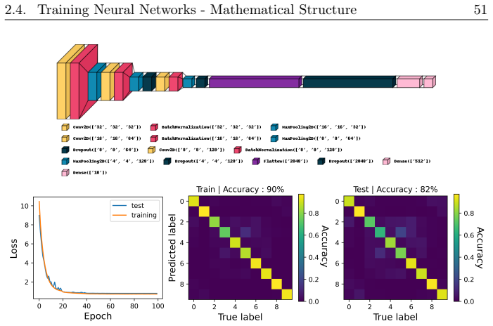
- [§2.3, §2.5.3] The numerical demonstrations are not reproducible from the text. No code, data, or random seeds are provided for the MNIST (Figs. 2.7–2.8), CIFAR-10 (Figs. 2.10, 2.13–2.15), or 2D Ising (Fig. 2.20) examples. Hyperparameters are incomplete or inconsistent: the MNIST experiment in §2.3.1 states η = 50, but §2.3.2 says 'same learning rate η = 1'; Fig. 2.7's caption says the input layer contains '282 nodes' where the text says 784. A student cannot reconstruct the claimed accuracies (56%, 95%, 82%, etc.) from the information given. This directly violates the preface's promise of 'hands-on examples' and weakens the pedagogical claim.
minor comments (7)
- [§2.2.2, Eq. (2.25)] The gradient-descent update is written as θ_{t+1} ← θ_t − η L(θ_t)/∂θ_t. The denominator should be ∂L(θ_t)/∂θ_t. As printed, the expression is not a valid derivative.
- [§2.3.1, Eq. (2.30)] The bias update line read 'b ← b − η ∂L/∂b = W − η ...'; the right-hand side should start with b, not W. This is a typo but confusing in a derivation.
- [§2.5.3] The Ising-model deep-learning demonstration does not cite the original works on machine-learning identification of phases (e.g., Carrasquilla and Melko, or related studies). For a set of lecture notes, this is a notable citation gap.
- [§3.6, Algorithm 4] The algorithm's input line says current RBM weights θ = {a, b, J}, while the text and Box 3.4 use W_{ij} for the coupling matrix. The notation should be unified.
- [§3.1.2, Eq. (3.7)] The t-SNE kernel is written as q_{ij} = (1 + ||y_i - y_j||^2)^{-1} / Σ_{k≠l}(1 + ||y_k - y_l||^2)^{-1}. The denominator should be normalized over ordered pairs (k,l) with k≠l, and the text should note that the numerator is the unnormalized Student-t kernel before division. This is minor but worth a clarifying sentence.
- [Various] There are many typographical and terminology issues: 'Principle Component Analysis' should be 'Principal Component Analysis'; 'Bolztmann' and 'Lecunn' are misspelled; Box 3.5 is labelled 'Box 3.4' in the text; 'mathematica' appears uncapitalized. None of these block the main points, but they should be cleaned up in a revision.
- [Box 2.6] The box calls the distance function a 'well defined metric' after listing only positivity and zero-on-equality. A metric also requires symmetry and the triangle inequality. The statement is mathematically imprecise.
Circularity Check
No circularity found: the notes are a tutorial that reproduces standard methods from external references; typos and internal inconsistencies do not constitute circular reasoning.
full rationale
The manuscript is a set of lecture notes, not an original derivation with predictions. Each technique (backpropagation, CNNs, VAEs, GANs, RBMs, normalising flows, Ising classification) is introduced from standard definitions and trained on data in the usual way. The Ising critical-temperature estimate is obtained by training a CNN on configurations labelled by phase (ordered vs disordered) while excluding the critical region, then locating the confidence minimum; the estimated Tc is a derived quantity and is not used as a training label, so the result does not reduce to its inputs by construction. The RBM partition function at Eq. (3.24) is misprinted as Z = sum_z E(z) instead of sum_z exp(-E(z)), and the subsequent derivation (Eqs. 3.36-3.39) uses the correct exponential form; this is an internal inconsistency/correctness issue, not a circular step. Likewise, the t-SNE KL-divergence remark and Eq. (2.5) dimension/bias-index mismatches are errata that undermine the pedagogical promise but do not make any claim equivalent to its own premise. The notes cite external literature for standard results; no load-bearing claim is justified solely by a self-citation. Therefore the circularity score is 0.
Assumptions & free parameters
assumptions (4)
- standard math Universal Approximation Theorem: a sufficiently wide or deep neural network can approximate any continuous function on a compact domain
- domain assumption Onsager's exact solution of the 2D Ising model: Tc = 2/ln(1+sqrt(2)) and exact magnetization/energy formulas
- standard math Shannon entropy convention H = -sum p log p
- domain assumption Manifold hypothesis: important features of high-dimensional data lie on a lower-dimensional manifold
Cite this review
Pith. "Pith review of Deep Learning in Classical and Quantum Physics." pith.science (2026). https://pith.science/paper/FEZABY5P
@misc{pith2026250810666,
  author       = {Pith},
  title        = {Pith review of: Deep Learning in Classical and Quantum Physics},
  year         = {2026},
  howpublished = {\url{https://pith.science/paper/FEZABY5P}},
  note         = {Machine review of arXiv:2508.10666}
}
read the original abstract
Scientific progress is tightly coupled to the emergence of new research tools. Today, machine learning (ML)-especially deep learning (DL)-has become a transformative instrument for quantum science and technology. Owing to the intrinsic complexity of quantum systems, DL enables efficient exploration of large parameter spaces, extraction of patterns from experimental data, and data-driven guidance for research directions. These capabilities already support tasks such as refining quantum control protocols and accelerating the discovery of materials with targeted quantum properties, making ML/DL literacy an essential skill for the next generation of quantum scientists. At the same time, DL's power brings risks: models can overfit noisy data, obscure causal structure, and yield results with limited physical interpretability. Recognizing these limitations and deploying mitigation strategies is crucial for scientific rigor. These lecture notes provide a comprehensive, graduate-level introduction to DL for quantum applications, combining conceptual exposition with hands-on examples. Organized as a progressive sequence, they aim to equip readers to decide when and how to apply DL effectively, to understand its practical constraints, and to adapt AI methods responsibly to problems across quantum physics, chemistry, and engineering.
Figures


Figures from the paper (61 more)




Forward citations
Cited by 1 Pith paper
-
Moment Optimization in the Navascu\'es-Pironio-Ac\'in Hierarchy
Budget-aware moment selection in the NPA hierarchy is a high-order combinatorial optimization problem where parallel tempering, an RBM-based policy, and Bayesian optimization all beat greedy selection, with the RBM cl...
Reference graph
Works this paper leans on
-
[1]
Turing Universality of the Game of Life, page 513–539
Paul Rendell. Turing Universality of the Game of Life, page 513–539. Springer London, 2002
2002
-
[2]
Myreen and Mario Carneiro
Magnus O. Myreen and Mario Carneiro. Gol in gol in hol: Verified circuits in conway’s game of life, 2025
2025
-
[3]
A. M. Turing. I.—computing machinery and intelligence. Mind, LIX(236):433–460, 10 1950
1950
-
[4]
Jack Copeland
B. Jack Copeland. Artificial Intelligence: A Philosophical Introduction. Blackwell, Cambridge, 1993
1993
-
[5]
Oxford University Press UK, 1999
Roger Penrose.Emperor’s New Mind. Oxford University Press UK, 1999
1999
-
[6]
Larson.The Myth of Artificial Intelligence: Why Computers Can’t Think the Way We Do
Erik J. Larson.The Myth of Artificial Intelligence: Why Computers Can’t Think the Way We Do. Harvard University Press, April 2021
2021
-
[7]
Sejnowski
Terrence J. Sejnowski. The Deep Learning Revolution. The MIT Press, 2018
2018
-
[8]
Artificial Life
Luc Steels and Rodney Brooks, editors. The "Artificial Life" Route to "Artificial Intelligence": Building Situated Embodied Agents. Hillsdale, NJ: Lawrence Erlbaum Associates, 1995
1995
Show all 105 references
-
[9]
Langton.Artificial Life: An Overview
Christopher G. Langton.Artificial Life: An Overview. MIT Press, Cam- bridge, MA, USA, 1st edition, 1995
1995
-
[10]
Introduction to artificial life
Christoph Adami. Introduction to artificial life. Springer-Verlag, Berlin, Heidelberg, 1999
1999
-
[11]
Chambers
Lance D. Chambers. Practical Handbook of Genetic Algorithms. CRC Press, Inc., USA, 1995
1995
-
[12]
Haupt.Frontmatter
Sue Ellen Haupt Randy L. Haupt.Frontmatter. John Wiley and Sons, Ltd, 2003
2003
-
[13]
Computational Intelligence
Leszek Rutkowski. Computational Intelligence. Springer Berlin Heidel- berg, 2008. 197 198 Bibliography
2008
-
[14]
Springer International Pub- lishing, 2017
Oliver Kramer.Genetic Algorithm Essentials. Springer International Pub- lishing, 2017
2017
-
[15]
Christopher M. Bishop. Pattern Recognition and Machine Learning (In- formation Science and Statistics). Springer-Verlag, Berlin, Heidelberg, 2006
2006
-
[16]
Shai Shalev-Shwartz and Shai Ben-David.Understanding Machine Learn- ing - From Theory to Algorithms.Cambridge University Press, 2014
2014
-
[17]
Witten, Eibe Frank, Mark A
Ian H. Witten, Eibe Frank, Mark A. Hall, and Christopher J. Pal.Data Mining, Fourth Edition: Practical Machine Learning Tools and Tech- niques. Morgan Kaufmann Publishers Inc., San Francisco, CA, USA, 4th edition, 2016
2016
-
[18]
Prince.Understanding Deep Learning
Simon J.D. Prince.Understanding Deep Learning. MIT Press, 2023
2023
-
[19]
Bishop and Hugh Bishop
Christopher M. Bishop and Hugh Bishop. Deep Learning: Foundations and Concepts. Springer International Publishing, 2024
2024
-
[20]
Machine learning and quantum devices.SciPost Phys
Florian Marquardt. Machine learning and quantum devices.SciPost Phys. Lect. Notes, page 29, 2021
2021
-
[21]
Ma- chine learning and the physical sciences.Rev
Giuseppe Carleo, Ignacio Cirac, Kyle Cranmer, Laurent Daudet, Maria Schuld, Naftali Tishby, Leslie Vogt-Maranto, and Lenka Zdeborová. Ma- chine learning and the physical sciences.Rev. Mod. Phys., 91:045002, Dec 2019
2019
-
[22]
Day, Clint Richardson, Charles K
Pankaj Mehta, Marin Bukov, Ching-Hao Wang, Alexandre G.R. Day, Clint Richardson, Charles K. Fisher, and David J. Schwab. A high-bias, low-variance introduction to machine learning for physicists.Physics Re- ports, 810:1–124, 2019. A high-bias, low-variance introduction to Mach...
2019
-
[23]
Michael Denner
Titus Neupert, Mark H Fischer, Eliska Greplova, Kenny Choo, and M. Michael Denner. Introduction to machine learning for the sciences, 2022
2022
-
[24]
Machine learning in quantum sciences
Anna Dawid, Julian Arnold, Borja Requena, Alexander Gresch, Marcin Płodzień, Kaelan Donatella, Kim A Nicoli, Paolo Stornati, Rouven Koch, Miriam Büttner, Robert Okuła, Gorka Muñoz-Gil, Rodrigo A Vargas- Hernández, Alba Cervera-Lierta, Juan Carrasquilla, Vedran Dunjko, Marylou ...
2025
-
[25]
Sadegh Raeisi and Sedighe Raeisi.Machine Learning for Physicists. 2053-
-
[26]
George V. Cybenko. Approximation by superpositions of a sigmoidal function. Mathematics of Control, Signals and Systems, 2:303–314, 1989
1989
-
[27]
Lecun, L
Y. Lecun, L. Bottou, Y. Bengio, and P. Haffner. Gradient-based learning applied to document recognition.Proceedings of the IEEE, 86(11):2278– 2324, 1998
1998
-
[28]
Introduction to Statistical Physics
Kerson Huang. Introduction to Statistical Physics . Chapman and Hall/CRC, September 2009
2009
-
[29]
Introduction: Classical phases and critical points
Jurgen Honig and Józef Spałek. Introduction: Classical phases and critical points. In A Primer to the Theory of Critical Phenomena, pages 1–8. Elsevier, 2018
2018
-
[30]
Bhattacharjee and Avinash Khare
Somendra M. Bhattacharjee and Avinash Khare. Fifty years of the exact solution of the two-dimensional ising model by onsager.Current Science, 69:816–820, 1995. Erratum: Current Science, 71 (1996) 493
1995
-
[31]
R. J. Baxter. Onsager and kaufman’s calculation of the sponta- neous magnetization of the ising model. Journal of Statistical Physics, 145(3):518–548, May 2011
2011
-
[32]
John R. Searle. Minds, brains, and programs. Behavioral and Brain Sciences, 3(3):417–424, September 1980
1980
-
[33]
Visualizing data using t-sne
Laurens Van der Maaten and Geoffrey Hinton. Visualizing data using t-sne. Journal of machine learning research, 9(11), 2008
2008
-
[34]
Learning deep architectures for ai, 2009
Y Bengio. Learning deep architectures for ai, 2009
2009
-
[35]
Auto-encoding variational bayes
Diederik P Kingma. Auto-encoding variational bayes. arXiv preprint arXiv:1312.6114, 2013
2013 arXiv
-
[36]
Normalizing flows on tori and spheres
Danilo Jimenez Rezende, George Papamakarios, Sébastien Racaniere, Michael Albergo, Gurtej Kanwar, Phiala Shanahan, and Kyle Cranmer. Normalizing flows on tori and spheres. In International Conference on Machine Learning, pages 8083–8092. PMLR, 2020
2020
-
[37]
Paulin de Schoulepnikoff, Gorka Muñoz-Gil, Hendrik Poulsen Nautrup, and Hans J. Briegel. Interpretable representation learning of quantum data enabled by probabilistic variational autoencoders. arXiv preprint arXiv: 2506.11982, 2025
2025
-
[38]
beta- vae: Learning basic visual concepts with a constrained variational frame- work
Irina Higgins, Loic Matthey, Arka Pal, Christopher Burgess, Xavier Glo- rot, Matthew Botvinick, Shakir Mohamed, and Alexander Lerchner. beta- vae: Learning basic visual concepts with a constrained variational frame- work. InInternational conference on learning representations,...
2017
-
[39]
Gener- ative adversarial nets.Advances in neural information processing systems, 27, 2014
Ian Goodfellow, Jean Pouget-Abadie, Mehdi Mirza, Bing Xu, David Warde-Farley, Sherjil Ozair, Aaron Courville, and Yoshua Bengio. Gener- ative adversarial nets.Advances in neural information processing systems, 27, 2014
2014
-
[40]
A learning algorithm for boltzmann machines.Cognitive science, 9(1):147–169, 1985
David H Ackley, Geoffrey E Hinton, and Terrence J Sejnowski. A learning algorithm for boltzmann machines.Cognitive science, 9(1):147–169, 1985
1985
-
[41]
“neural” computation of decisions in optimization problems
John J Hopfield and David W Tank. “neural” computation of decisions in optimization problems. Biological cybernetics, 52(3):141–152, 1985
1985
-
[42]
Anna Dawid and Yann LeCun. Introduction to latent variable energy- based models: a path toward autonomous machine intelligence.Journal of Statistical Mechanics: Theory and Experiment, 2024(10):104011, October 2024
2024
-
[43]
Hitchhiker’sguideontherelationofenergy-basedmodels with other generative models, sampling and statistical physics: a compre- hensive review, 2024
DavideCarbone. Hitchhiker’sguideontherelationofenergy-basedmodels with other generative models, sampling and statistical physics: a compre- hensive review, 2024
2024
-
[44]
Normalizing flows for proba- bilistic modeling and inference
George Papamakarios, Eric Nalisnick, Danilo Jimenez Rezende, Shakir Mohamed, and Balaji Lakshminarayanan. Normalizing flows for proba- bilistic modeling and inference. Journal of Machine Learning Research, 22(57):1–64, 2021
2021
-
[45]
A universal approximation theorem of deep neural networks for expressing probability distributions.Advances in neu- ral information processing systems, 33:3094–3105, 2020
Yulong Lu and Jianfeng Lu. A universal approximation theorem of deep neural networks for expressing probability distributions.Advances in neu- ral information processing systems, 33:3094–3105, 2020
2020
-
[46]
Normalizing flows: An introduction and review of current methods.IEEE transactions on pattern analysis and machine intelligence, 43(11):3964–3979, 2020
Ivan Kobyzev, Simon JD Prince, and Marcus A Brubaker. Normalizing flows: An introduction and review of current methods.IEEE transactions on pattern analysis and machine intelligence, 43(11):3964–3979, 2020
2020
-
[47]
Physics- informed neural networks: A deep learning framework for solving forward and inverse problems involving nonlinear partial differential equations
Maziar Raissi, Paris Perdikaris, and George E Karniadakis. Physics- informed neural networks: A deep learning framework for solving forward and inverse problems involving nonlinear partial differential equations. Journal of Computational physics, 378:686–707, 2019
2019
-
[48]
Explaining quantum circuits with shap- ley values: Towards explainable quantum machine learning
Raoul Heese, Thore Gerlach, Sascha Mücke, Sabine Müller, Matthias Jakobs, and Nico Piatkowski. Explaining quantum circuits with shap- ley values: Towards explainable quantum machine learning. Quantum Machine Intelligence, 7(1):1–33, 2025
2025
-
[49]
Causability and explainability of artificial intelligence in medicine
Andreas Holzinger, Georg Langs, Helmut Denk, Kurt Zatloukal, and Heimo Müller. Causability and explainability of artificial intelligence in medicine. Wiley Interdisciplinary Reviews: Data Mining and Knowledge Discovery, 9(4):e1312, 2019
2019
-
[50]
Beyond human: Deep learning, explainability and rep- resentation
M Beatrice Fazi. Beyond human: Deep learning, explainability and rep- resentation. Theory, Culture & Society, 38(7-8):55–77, 2021. 200 Bibliography 201
2021
-
[51]
On the interpretability of quantum neural networks
Lirandë Pira and Chris Ferrie. On the interpretability of quantum neural networks. Quantum Machine Intelligence, 6(2):52, 2024
2024
-
[52]
Interpretable deep learning: Interpretation, interpretability, trustworthiness, and beyond.Knowledge and Information Systems, 64(12):3197–3234, 2022
Xuhong Li, Haoyi Xiong, Xingjian Li, Xuanyu Wu, Xiao Zhang, Ji Liu, Jiang Bian, and Dejing Dou. Interpretable deep learning: Interpretation, interpretability, trustworthiness, and beyond.Knowledge and Information Systems, 64(12):3197–3234, 2022
2022
-
[53]
Visual interpretability for deep learning: a survey.Frontiers of Information Technology & Electronic En- gineering, 19(1):27–39, 2018
Quan-shi Zhang and Song-Chun Zhu. Visual interpretability for deep learning: a survey.Frontiers of Information Technology & Electronic En- gineering, 19(1):27–39, 2018
2018
-
[54]
Cambridge university press, 2010
Michael A Nielsen and Isaac L Chuang.Quantum computation and quan- tum information. Cambridge university press, 2010
2010
-
[55]
Cambridge university press, 2018
David J Griffiths and Darrell F Schroeter.Introduction to quantum me- chanics. Cambridge university press, 2018
2018
-
[56]
John Wiley & Sons, 2015
Wolfgang P Schleich.Quantum optics in phase space. John Wiley & Sons, 2015
2015
-
[57]
John Wiley & Sons, 2009
Andrei B Klimov and Sergei M Chumakov.A group-theoretical approach to quantum optics: models of atom-field interactions. John Wiley & Sons, 2009
2009
-
[58]
Springer, 2018
Bernard Zygelman.A first introduction to quantum computing and infor- mation. Springer, 2018
2018
-
[59]
Springer Science & Business Media, 2009
Gregg Jaeger.Entanglement, information, and the interpretation of quan- tum mechanics. Springer Science & Business Media, 2009
2009
-
[60]
A brief introduction to multi- partite entanglement.arXiv preprint arXiv:1612.07747, 2016
Ingemar Bengtsson and Karol Zyczkowski. A brief introduction to multi- partite entanglement.arXiv preprint arXiv:1612.07747, 2016
2016 arXiv
-
[61]
Cambridge University Press, May 2006
Ingemar Bengtsson and Karol Zyczkowski.Geometry of Quantum States: An Introduction to Quantum Entanglement. Cambridge University Press, May 2006
2006
-
[62]
A short review on entanglement in quan- tum spin systems
J I Latorre and A Riera. A short review on entanglement in quan- tum spin systems. Journal of Physics A: Mathematical and Theoretical, 42(50):504002, December 2009
2009
-
[63]
Quantum entanglement
Ryszard Horodecki, Paweł Horodecki, Michał Horodecki, and Karol Horodecki. Quantum entanglement. Reviews of Modern Physics , 81(2):865–942, June 2009
2009
-
[64]
Springer Nature Switzerland, 2024
Anubhav Kumar Srivastava, Guillem Müller-Rigat, Maciej Lewenstein, and Grzegorz Rajchel-Mieldzioć.Introduction to Quantum Entanglement in Many-Body Systems, page 225–285. Springer Nature Switzerland, 2024. 201 202 Bibliography
2024
-
[65]
Multipartite entanglement
Pawel Horodecki, Łukasz Rudnicki, and Karol Zyczkowski. Multipartite entanglement. arXiv, 2024
2024
-
[66]
En- tangling power of multipartite unitary gates.Journal of Physics A: Math- ematical and Theoretical, 53(12):125303, March 2020
TomaszLinowski, GrzegorzRajchel-Mieldzioć, andKarolŻyczkowski. En- tangling power of multipartite unitary gates.Journal of Physics A: Math- ematical and Theoretical, 53(12):125303, March 2020
2020
-
[67]
Introduction to haar measure tools in quantum in- formation: A beginner’s tutorial.Quantum, 8:1340, May 2024
Antonio Anna Mele. Introduction to haar measure tools in quantum in- formation: A beginner’s tutorial.Quantum, 8:1340, May 2024
2024
-
[68]
Predicting many properties of a quantum system from very few measurements
Hsin-Yuan Huang, Richard Kueng, and John Preskill. Predicting many properties of a quantum system from very few measurements. Nature Physics, 16(10):1050–1057, June 2020
2020
-
[69]
Struchalin, Ya
G.I. Struchalin, Ya. A. Zagorovskii, E.V. Kovlakov, S.S. Straupe, and S.P. Kulik. Experimental estimation of quantum state properties from classical shadows. PRX Quantum, 2(1), January 2021
2021
-
[70]
Learning quantum states from their classical shadows
Hsin-Yuan Huang. Learning quantum states from their classical shadows. Nature Reviews Physics, 4(2):81–81, January 2022
2022
-
[71]
GitHub Repo
Marcin Płodzień. Quantum-State-Tomography-with-Classical-Shadows- from-scratch. "GitHub Repo", February 2023
2023
-
[72]
Quantum machine learning in multi-qubit phase- space part i: Foundations.arXiv preprint arXiv:2507.12117, 2025
Timothy Heightman, Edward Jiang, Ruth Mora-Soto, Maciej Lewenstein, and Marcin Płodzień. Quantum machine learning in multi-qubit phase- space part i: Foundations.arXiv preprint arXiv:2507.12117, 2025
2025
-
[73]
Entanglement classification and non- k -separability certification via Greenberger-Horne-Zeilinger-class fidelity
Marcin Płodzień, Jan Chwedeńczuk, Maciej Lewenstein, and Grzegorz Rajchel-Mieldzioć. Entanglement classification and non- k -separability certification via Greenberger-Horne-Zeilinger-class fidelity. Physical Re- view A, 110(3), September 2024
2024
-
[74]
Oxford Univer- sity Press, 12 2003
Thierry Giamarchi.Quantum Physics in One Dimension. Oxford Univer- sity Press, 12 2003
2003
-
[75]
Introduction to quantum integrability
Jules Lamers. Introduction to quantum integrability. In Proceed- ings of 10th Modave Summer School in Mathematical Physics — PoS(Modave2014), Modave2014, page001.SissaMedialab, February2015
-
[76]
An Introduction to Integrable Techniques for One- Dimensional Quantum Systems
Fabio Franchini. An Introduction to Integrable Techniques for One- Dimensional Quantum Systems. Springer International Publishing, 2017
2017
-
[77]
A variational eigenvalue solver on a photonic quantum processor.Nature communications, 5(1):4213, 2014
Alberto Peruzzo, Jarrod McClean, Peter Shadbolt, Man-Hong Yung, Xiao-Qi Zhou, Peter J Love, Alán Aspuru-Guzik, and Jeremy L O’brien. A variational eigenvalue solver on a photonic quantum processor.Nature communications, 5(1):4213, 2014
2014
-
[78]
Geometry of variational methods: dynamics of closed quantum systems.SciPost Physics, 9(4):048, 2020
Lucas Hackl, Tommaso Guaita, Tao Shi, Jutho Haegeman, Eugene Dem- ler, and J Ignacio Cirac. Geometry of variational methods: dynamics of closed quantum systems.SciPost Physics, 9(4):048, 2020. 202 Bibliography 203
2020
-
[79]
Quan- tum natural gradient.Quantum, 4:269, 2020
James Stokes, Josh Izaac, Nathan Killoran, and Giuseppe Carleo. Quan- tum natural gradient.Quantum, 4:269, 2020
2020
-
[80]
Princeton University Press, 2021
Tristan Needham.Visual differential geometry and forms: a mathematical drama in five acts. Princeton University Press, 2021
2021
-
[81]
Springer, 1996
Anthony W Knapp and Anthony William Knapp.Lie groups beyond an introduction, volume 140. Springer, 1996
1996
-
[82]
A unified theory of barren plateaus for deep parametrized quantum circuits.arXiv preprint arXiv:2309.09342, 2023
Michael Ragone, Bojko N Bakalov, Frédéric Sauvage, Alexander F Kem- per, Carlos Ortiz Marrero, Martin Larocca, and M Cerezo. A unified theory of barren plateaus for deep parametrized quantum circuits.arXiv preprint arXiv:2309.09342, 2023
2023 arXiv
-
[83]
Showcasing a barren plateau theory beyond the dynamical lie algebra
NL Diaz, Diego García-Martín, Sujay Kazi, Martin Larocca, and M Cerezo. Showcasing a barren plateau theory beyond the dynamical lie algebra. arXiv preprint arXiv:2310.11505, 2023
2023 arXiv
-
[84]
A review of barren plateaus in variational quan- tum computing
Martin Larocca, Supanut Thanasilp, Samson Wang, Kunal Sharma, Ja- cob Biamonte, Patrick J Coles, Lukasz Cincio, Jarrod R McClean, Zoë Holmes, and M Cerezo. A review of barren plateaus in variational quan- tum computing. arXiv preprint arXiv:2405.00781, 2024
2024 arXiv
-
[85]
A quantum approx- imate optimization algorithm.arXiv preprint arXiv:1411.4028, 2014
Edward Farhi, Jeffrey Goldstone, and Sam Gutmann. A quantum approx- imate optimization algorithm.arXiv preprint arXiv:1411.4028, 2014
2014 arXiv
-
[86]
Solving the quantum many-body problem with artificial neural networks.Science, 355(6325):602–606, 2017
Giuseppe Carleo and Matthias Troyer. Solving the quantum many-body problem with artificial neural networks.Science, 355(6325):602–606, 2017
2017
-
[87]
From architectures to applications: A review of neural quantum states
Hannah Lange, Anka Van de Walle, Atiye Abedinnia, and Annabelle Bohrdt. From architectures to applications: A review of neural quantum states. Quantum Science and Technology, 2024
2024
-
[88]
On neural differential equations
Patrick Kidger. On neural differential equations. arXiv preprint arXiv:2202.02435, 2022
2022 arXiv
-
[89]
Solving the quan- tum many-body hamiltonian learning problem with neural differential equations
Timothy Heightman, Edward Jiang, and Antonio Acín. Solving the quan- tum many-body hamiltonian learning problem with neural differential equations. arXiv preprint arXiv:2408.08639, 2024
2024 arXiv
-
[90]
Quantum error correction below the surface code threshold
Google Quantum AI et al. Quantum error correction below the surface code threshold. Nature, 638(8052):920, 2024
2024
-
[91]
Universal quantum control through deep reinforcement learning
Murphy Yuezhen Niu, Sergio Boixo, Vadim N Smelyanskiy, and Hartmut Neven. Universal quantum control through deep reinforcement learning. npj Quantum Information, 5(1):33, 2019
2019
-
[92]
MIT press Cambridge, 1998
Richard S Sutton, Andrew G Barto, et al.Reinforcement learning: An introduction, volume 1. MIT press Cambridge, 1998. 203 204 Bibliography
1998
-
[93]
Enhancing quantum state tomography via resource-efficient attention-based neural networks.Physical Review Research, 6(3), Septem- ber 2024
Adriano Macarone Palmieri, Guillem Müller-Rigat, Anubhav Kumar Sri- vastava, Maciej Lewenstein, Grzegorz Rajchel-Mieldzioć, and Marcin Płodzień. Enhancing quantum state tomography via resource-efficient attention-based neural networks.Physical Review Research, 6(3), Septem- ber 2024
2024
-
[94]
Natural gradient works efficiently in learning.Neural computation, 10(2):251–276, 1998
Shun-Ichi Amari. Natural gradient works efficiently in learning.Neural computation, 10(2):251–276, 1998
1998
-
[95]
New insights and perspectives on the natural gradient method
James Martens. New insights and perspectives on the natural gradient method. Journal of Machine Learning Research, 21(146):1–76, 2020
2020
-
[96]
Daniel Freeman, Theodore R
Adly Templeton, Tom Conerly, Jonathan Marcus, Jack Lindsey, Trenton Bricken, Brian Chen, Adam Pearce, Craig Citro, Emmanuel Ameisen, Andy Jones, Hoagy Cunningham, Nicholas L Turner, Callum McDougall, MonteMacDiarmid, AlexTamkin, EsinDurmus, TristanHume, Francesco Mosconi, C. D...
2024
-
[97]
Graph of thoughts: Solving elabo- rate problems with large language models
Maciej Besta, Nils Blach, Ales Kubicek, Robert Gerstenberger, Michal Podstawski, Lukas Gianinazzi, Joanna Gajda, Tomasz Lehmann, Hubert Niewiadomski, Piotr Nyczyk, et al. Graph of thoughts: Solving elabo- rate problems with large language models. InProceedings of the AAAI Conf...
2024
-
[98]
Large language models are in-context semantic reasoners rather than symbolic reasoners
Xiaojuan Tang, Zilong Zheng, Jiaqi Li, Fanxu Meng, Song-Chun Zhu, Yitao Liang, and Muhan Zhang. Large language models are in-context semantic reasoners rather than symbolic reasoners. arXiv preprint arXiv:2305.14825, 2023
2023 arXiv
-
[99]
World of patterns
RensBod. World of patterns. A global history of knowledge. JohnsHopkins University Press, Baltimore, MD, July 2022
2022
-
[100]
Geometric deep learning: Grids, groups, graphs, geodesics, and gauges
Michael M Bronstein, Joan Bruna, Taco Cohen, and Petar Veličković. Geometric deep learning: Grids, groups, graphs, geodesics, and gauges. arXiv preprint arXiv:2104.13478, 2021
2021 arXiv
-
[101]
Mathematical founda- tions of geometric deep learning.arXiv preprint arXiv:2508.02723, 2025
Haitz Sáez de Ocáriz Borde and Michael Bronstein. Mathematical founda- tions of geometric deep learning.arXiv preprint arXiv:2508.02723, 2025
2025 arXiv
-
[102]
Springer, 2021
Maria Schuld and Francesco Petruccione.Machine learning with quantum computers, volume 676. Springer, 2021
2021
-
[103]
Matthias Klusch, Jörg Lässig, Daniel Müssig, Antonio Macaluso, and Frank K. Wilhelm. Quantum artificial intelligence: A brief survey. KI - Künstliche Intelligenz, 38(4):257–276, November 2024. 204 Bibliography 205
2024
-
[104]
Andrew D
Giovanni Acampora, Andris Ambainis, Natalia Ares, Leonardo Banchi, Pallavi Bhardwaj, Daniele Binosi, G. Andrew D. Briggs, Tommaso Calarco, Vedran Dunjko, Jens Eisert, Olivier Ezratty, Paul Erker, Fed- erico Fedele, Elies Gil-Fuster, Martin Gärttner, Mats Granath, Markus Heyl, ...
2025
-
[2563]
198 Bibliography 199
IOP Publishing, 2023. 198 Bibliography 199
2023
Reviewed August 5, 2026 · model on record in the stance chip above.
Discussion (0). Sign in to comment.