REVIEW 3 major objections 5 minor 31 references
Grokking Beyond the Euclidean Norm of Model Parameters
T0 review · 3 major / 5 minor · reviewed 2026-08-07 · deepseek-v4-flash
Pith's one-line read Grokking is a generic effect of any regularizer that biases toward a generalizing structure, with the delay set by the product of learning rate and regularization strength.
desk verdict A real extension of grokking theory beyond ℓ2, but the headline 1/(αβ) delay law is proven only as an upper bound and the 'iff' statements outrun the appendix. read the letter →
The pith
A machine-rendered reading of the paper's core claim, the machinery that carries it, and where it could break.
The reading
What carries the argument
The load-bearing object is the two-phase decomposition of subgradient descent on the composite objective $g + \beta h$. The first phase is controlled by the $r$-Chatterjee–Łojasiewicz inequality at initialization, $4g(x(0)) < r^2\chi(g, x(0), r)$, which guarantees geometric decay of the loss while iterates stay inside a ball; the condition $\beta\lVert H(x(k))\rVert_2 \leq \gamma\lVert G(x(k))\rVert_2$ ensures the regularizer does not interfere until the loss is nearly minimized. The second phase is governed by the distance-to-set identity $\Delta t = \mathrm{dist}^2(x(t_1), \Theta_f)/(\alpha\beta\eta)$, the ratio of the squared distance from the memorizing iterate to the regularized solution set and the step $\alpha\beta\eta$; this is what makes the grokking delay inversely proportional to $\alpha\beta$. In the linear settings, the robust null space property (or its rank analogue) converts near-equality of the $\ell_1$ (or nuclear) norm with the target into near-recovery of the true solution, closing the loop between regularization and generalization, while the Wedin $\sin\Theta$ bound controls the drift of singular vectors during the late phase.
What would settle it
On a sparse recovery instance where the design matrix satisfies the null space property and the CL condition holds at initialization, vary $\alpha$ and $\beta$ independently over two orders of magnitude and measure the step at which the recovery error first drops below a fixed threshold; if doubling $\alpha$ alone does not halve the required extra time $\Delta t$, the claimed $1/(\alpha\beta)$ scaling is false. A complementary test is to initialize a two-layer ReLU teacher-student at a point where the CL inequality is violated (a flat loss region) and run with small $\ell_1$ regularization; observing grokking there would show the CL condition is not necessary.
Extended reading notes
Core claim
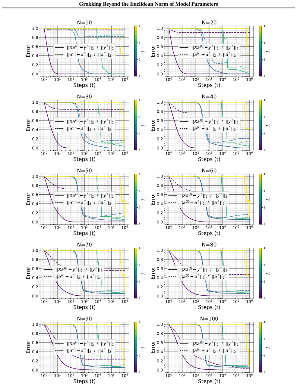
On the paper's own terms, the central discovery is that regularized subgradient descent exhibits a provable two-phase dynamic whenever the loss satisfies the Chatterjee–Łojasiewicz inequality at its initialization and the regularization term stays dominated by the loss gradient throughout the first phase. In that setting the iterates first reach an almost-interpolating (memorizing) solution in about $t_1 \approx O\!\left(\log(1/\varepsilon)/\alpha\chi\right)$ steps, and then need an additional $\Delta t \approx \mathrm{dist}^2(x(t_1), \Theta_f)/(\alpha\beta\eta)$ steps to approach the minimizer of the regularized objective, with recovery error of order $O(\alpha\beta + \lVert \xi \rVert)$. For sparse recovery and low-rank matrix sensing and completion, the paper proves that this delay law holds, that the $\ell_1$ or nuclear-norm regularizer is necessary in the shallow case (weight decay alone only yields a memorizing least-squares solution), and that depth or coherence-based data selection can supply the same bias implicitly. The paper further documents, on modular addition and image classification, that $\ell_1$ and nuclear-norm regularization reproduce the grokking curves previously attributed to $\ell_2$, and that the $\ell_2$ norm can rise while generalization is happening.
Load-bearing premise
The clean delay law rests on the loss satisfying the Chatterjee–Łojasiewicz inequality at the exact initialization and on the regularizer's subgradient staying much weaker than the loss gradient until memorization; for nonlinear teacher-student, modular arithmetic, and image data this condition is imported from wide-network theory rather than verified, and the noiseless alignment $\Theta_f \cap \Theta_g \neq \varnothing$ together with the noise bound $\lVert X^\top\xi \rVert_2 \leq \sqrt{C\alpha\beta}$ restricts the $1/(\alpha\beta)$ law to an essentially noiseless regime.
Editorial extensions
If this is right
- If the central theorem is right, grokking should be reproducible with any regularizer whose bias is aligned with the structure of a good solution—sparsity, low rank, or a domain constraint—and the delay is predictable from $\alpha\beta$ alone.
- Weight decay is not a necessary condition for grokking, and a decreasing $\ell_2$ norm is not a necessary signature; monitoring the norm of the regularized property, such as the $\ell_1$ or nuclear norm, is the better progress signal.
- Depth acts as an implicit regularizer that can replace explicit $\ell_1$ or nuclear-norm penalties: deeper linear models grok without explicit regularization in the sparse and low-rank settings studied, and can even un-grok when the bias is no longer needed.
- Choosing training samples with high leverage scores (coherence) relative to the target low-rank or sparse structure can cut both the number of examples needed and the time to generalization, and this can be done with all other hyperparameters fixed.
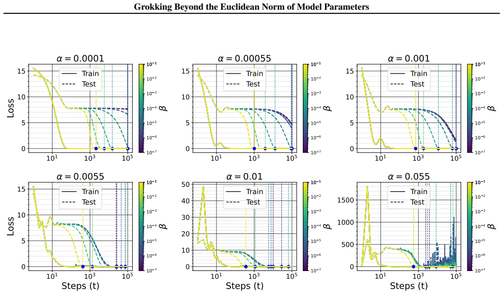
- The scaling $\Delta t \propto 1/(\alpha\beta)$ gives a quantitative handle for scheduling: increasing $\alpha\beta$ accelerates generalization, while keeping it small produces the long delayed-generalization window associated with grokking.
Reading between the lines
- Editorial inference: the theory suggests a practical recipe for inducing grokking in any overparameterized model—identify the known structure of the desired solution, add a small penalty toward it, and tune the delay a priori through the product of learning rate and penalty strength.
- Editorial inference: the two-phase mechanism closely parallels circuit-competition accounts of grokking; if the late-phase bias is the circuit-selection force, the same $1/(\alpha\beta)$ delay law should appear whenever a slow second-order drift pushes weights from a kernel-like to a structured solution, connecting to feature-learning theories of grokking.
- Editorial inference: the coherence-based data selection result yields a testable extension—on modular arithmetic or low-rank tasks, training on highest-leverage-score entries should shift the grokking curve left relative to uniform sampling even at a fixed total sample count.
- Editorial inference: because the $\ell_2$ norm can rise with generalization, previously reported norm-decrease or slingshot phenomena should be re-examined under $\ell_1$ and nuclear regularization; the same phase transition may be visible in the $\ell_1$ or nuclear norm instead.
Editorial analysis
A structured set of objections, weighed in public.
Referee Report
Summary. The paper develops a general theory of grokking as a two-phase phenomenon induced by regularization toward a property P (sparsity, low rank), with a main theorem claiming that after a memorization phase the generalization delay is Δt = dist²(x(t1), Θf)/(αβη) for step size α and regularization strength β. It instantiates this for sparse recovery with ℓ1 regularization and for matrix factorization with nuclear-norm regularization, and it provides extensive experiments on modular arithmetic, teacher-student networks, MNIST, data selection, and depth. It also reports that the ℓ2 norm can rise during generalization when ℓ1/ℓ∗ regularization is used, and it identifies a failure mode called 'grokking without understanding' under large initialization with weight decay.
Significance. If the main theorem's quantitative claim were fully proven, the paper would be a substantial extension of Lyu et al. (2023) and would provide a unifying explanation for regularization-induced grokking beyond ℓ2. The paper's parameter-free delay formula (no fitted constants), its explicit instantiations in linear sparse/low-rank settings, and its broad empirical validation with reproducible code are genuine strengths. The experiments sweeping α and β and reporting t2 ∝ 1/(αβ) are valuable even if the theory currently establishes only an upper bound; however, the missing lower bound in the central theorem means that the headline claim that the delay 'scales like 1/(αβ)' is not yet proven.
major comments (3)
- [Theorem 2.1 and Appendix C.1 (Lemma C.12, Theorem C.13)] The 'if and only if' in the second bullet is not established by the proof. Lemma C.12 gives an upper bound on min_{t1≤t≤t2}(f(x(t))−f*), and Theorem C.13 combines it with max∥F∥²≤Cβ² to obtain the implication t2−t1≥R²/(αβη) ⇒ min≤(η+Cαβ)β/2. This is a sufficient condition only; a matching lower bound would require a converse inequality (e.g., a uniform lower bound on ∥F(x(t))∥ or on the rate of decrease of dist(x(t),Θf)), which is not supplied. Since the abstract and Section 2 state the delay 'scales like 1/(αβ)' as an equality-type law, this gap is load-bearing for the paper's central claim. Please either prove the lower bound or restate the theorem as an upper-bound/sufficient condition.
- [Theorems 3.1, 3.3, 3.4, 3.5 and proofs C.4–C.7] These results inherit the same unsupported 'iff'. Theorem 3.1 is proved by invoking Theorem C.13, and Theorems 3.3 and 3.5 only add the robust null space or rank null space property on top of that; consequently, the recovery-error statements also hold only as sufficient conditions. The exact thresholds in Lemmas C.31 and C.42 are derived for the pure shrinkage dynamics a_{t+1}=a_t−αβH(a_t) (or, in the matrix case, for the polar subgradient H=UV⊤), but in the actual dynamics (1) the loss gradient G(x(t)) is present and arbitrary subgradient selections are allowed, so those lemmas do not provide the missing lower bound for the full dynamics. Furthermore, for a general H∈∂∥A∥*, the −αW term in the nuclear-norm subgradient can change the singular values beyond the claimed |σ_i−α|, so Lemma C.42 is not valid for arbitrary subgradient selections. The empirical scaling in Figures 4 and 6 supports 1/(αβ) but does not fill this logical gap.
- [Section 4 and Theorem 2.1 assumptions] Theorem 2.1 is conditional on g being r-CL at initialization and on β∥H(x(k))∥₂ staying dominated by ∥G(x(k))∥₂ throughout the memorization phase; these conditions are cited from Liu et al. (2021) for wide overparameterized networks but are not verified for the nonlinear teacher-student, modular arithmetic, or MNIST models used in Section 4. The paper should state explicitly that for these models the theoretical delay law is a conjecture supported by experiments, not a theorem.
minor comments (5)
- [Theorem 2.1 vs Theorem C.13] Theorem 2.1 writes 't2 > t1 + Δt' while Theorem C.13 and the proofs use 't2 ≥ t1 + Δt'; please make the threshold inequalities consistent across the statements.
- [Throughout the text] Typos such as 'coefficent', 'ovaparametrization', 'Cohence', and 'they Assumption 3.2' should be corrected.
- [Figure 1 caption] The bottom caption says 'In the case of ℓ1 (top-left)' while referring to bottom panels; please clarify which panel shows which norm dynamics.
- [Section 3.5 (Implicit Bias of the Depth)] The notation a = ⊙_{k=1}^L A_k is used without defining the per-layer domain or the corresponding gradient update; please specify A_k ∈ R^n (or the matrix form) and the update rule for the deep parameterization.
- [References] At least one bibliography entry contains raw HTML entities such as 'ℓ'; these should be cleaned up for publication.
Circularity Check
No significant circularity: the derived 1/(alpha*beta) delay law uses no fitted constants, and the generalization bridge is external compressed-sensing theory.
full rationale
The paper's central quantitative claim is the delay formula Delta_t = dist^2(x(t1), Theta_f)/(alpha*beta*eta). This quantity is derived in Theorem C.13 and Lemma C.12 from the subgradient descent recurrence and the bound ||F(x(t))||^2 = O(beta^2); it contains no fitted parameter later relabeled as a prediction. The experiments sweep alpha and beta and compare against the computed t2, rather than fitting the 1/(alpha*beta) scaling. The bridge from minimizing h over Theta_g to generalization is supplied by external compressed-sensing results (robust null space property and Wedin sin-Theta bounds), not by a self-citation chain. The Chatterjee-Lojasiewicz regularity assumption is cited from Liu et al. (2021), not from the present authors' prior work, and is an assumption about the loss landscape rather than a restatement of the conclusion. The self-reference to Notsawo et al. (2023) appears only in the related-work survey and is not load-bearing. The proof's 'if and only if' in Theorem 2.1 and its instantiations is not actually established by the displayed upper-bound inequality in Lemma C.12; this is a correctness gap about a missing lower bound, not a circular reduction of the prediction to its inputs. No step in the derivation is, by the paper's own equations, equivalent to its input by construction.
Assumptions & free parameters
free parameters (3)
- initialization scale ζ (deep sparse recovery) =
ζ = 1e-6 (L=1), ζ = 1e-2 (L>1); large ζ = 10 for ℓ2 experiments
- sparse recovery configuration (n, s, N, α, β) =
(102, 5, 30, 1e-1, 1e-5)
- matrix completion configuration (n1, n2, r, N, α, β) =
(10, 10, 2, 70, 1e-1, 1e-4)
assumptions (5)
- domain assumption g satisfies the r-CL inequality at initialization: 4g(x(0)) < r²χ(g, x(0), r)
- domain assumption Assumption C.5: Θf ∩ Θg ≠ ∅
- domain assumption Noise bound ∥X⊤ξ∥₂ ≤ √(Cαβ)
- domain assumption Robust null space property / robust rank null space property of the measurement map
- standard math Step-size and regularization bounds: 0 < ασmax(X⊤X) < 2, 0 < β√n < σmax(X⊤X)
Cite this review
Pith. "Pith review of Grokking Beyond the Euclidean Norm of Model Parameters." pith.science (2026). https://pith.science/paper/JUZYCOJ5
@misc{pith2026250605718,
  author       = {Pith},
  title        = {Pith review of: Grokking Beyond the Euclidean Norm of Model Parameters},
  year         = {2026},
  howpublished = {\url{https://pith.science/paper/JUZYCOJ5}},
  note         = {Machine review of arXiv:2506.05718}
}
abstract
Grokking refers to a delayed generalization following overfitting when optimizing artificial neural networks with gradient-based methods. In this work, we demonstrate that grokking can be induced by regularization, either explicit or implicit. More precisely, we show that when there exists a model with a property $P$ (e.g., sparse or low-rank weights) that generalizes on the problem of interest, gradient descent with a small but non-zero regularization of $P$ (e.g., $\ell_1$ or nuclear norm regularization) results in grokking. This extends previous work showing that small non-zero weight decay induces grokking. Moreover, our analysis shows that over-parameterization by adding depth makes it possible to grok or ungrok without explicitly using regularization, which is impossible in shallow cases. We further show that the $\ell_2$ norm is not a reliable proxy for generalization when the model is regularized toward a different property $P$, as the $\ell_2$ norm grows in many cases where no weight decay is used, but the model generalizes anyway. We also show that grokking can be amplified solely through data selection, with any other hyperparameter fixed.
Figures


Figures from the paper (31 more)






Reference graph
Works this paper leans on
-
[1]
We also have ∥zy∥2 ≤ L since L = supy′∈B(x,r) supz∈∂h(y′) ∥z∥2
If g(y) ̸= 04, then since y ∈ B(x, r) and g(y) ̸= 0, we have ∥∇g(y)∥2 2 ≥ g(y) · χ(g, x, r) from the CL constant for g. We also have ∥zy∥2 ≤ L since L = supy′∈B(x,r) supz∈∂h(y′) ∥z∥2. Using Cauchy–Schwarz: ⟨∇g(y), zy⟩ ≥ −∥∇g(y)∥2 · ∥zy∥2 ≥ −L∥∇g(y)∥2 (58) So ∥∇f (y)∥2 2 = ∥∇g(y)∥2 2 + 2β⟨∇g(y), zy⟩ + β2∥zy∥2 2 ≥ ∥∇g(y)∥2 2 + 2β⟨∇g(y), zy⟩ ≥ ∥∇g(y)∥2 2 − 2...
-
[2]
Then, for any η >0, mint1≤t≤t2 f (x(t)) − f ∗ ≤ (η+Cαβ )β 2 if and only if t2 ≥ t1 + R2 αβη
Assume there exists a constant C >0, L ≤ Cβ 2. Then, for any η >0, mint1≤t≤t2 f (x(t)) − f ∗ ≤ (η+Cαβ )β 2 if and only if t2 ≥ t1 + R2 αβη . Moreover, if Assumptions C.5 holds, then mint1≤t≤t2 h(x(t)) − h∗ g ≤ η+Cαβ 2 if and only if t2 ≥ t1 + R2 αβη . Proof. Using maxt1≤t≤t2 ∥F (x(t))∥2 2 ≤ maxt1≤t ∥F (x(t))∥2 2 = L ≤ Cβ 2, we derive the following from Le...
work page 2022
-
[3]
In particular, for h(a) = sign(a) ∀a ∈ R, if a(1)/α ∈ Z, then a(t) = 0 for all t >⌊ |a(1)| α ⌋. Proof. Let first consider the simple case H(a) = sign(a), so that a(t+1) = a(t) − α sign(a(t)). • If a(t) ∈ {0, α,−α}, then a(t+∆) = 0 for all ∆ > 0. • If a(t) ∈ (0, α), then a(t+1) = a(t) − α ∈ (−α, 0), and a(t+2) = a(t+1) + α = a(t) ∈ (0, α), and so on. • If ...
-
[6]
Unveiling the Dynamics of Information Interplay in Supervised Learning
URL https://proceedings.neurips. cc/paper_files/paper/1996/file/ e1d5be1c7f2f456670de3d53c7b54f4a-Paper. pdf. Saad, D. and Solla, S. A. On-line learning in soft committee machines. Phys. Rev. E, 52:4225–4243, Oct 1995a. doi: 10.1103/PhysRevE.52.4225. URL https://link. aps.org/doi/10.1103/PhysRevE.52.4225. Saad, D. and Solla, S. A. Exact solution for on-li...
work page Pith review arXiv 1996
-
[9]
https://www.stat.cmu.edu/˜ryantibs/ convexopt-S15/, 2015. Tsang, I. W., Kwok, J. T., and Cheung, P.-M. Core vec- tor machines: Fast svm training on very large data sets. Journal of Machine Learning Research, 6(13):363– 392, 2005. URL http://jmlr.org/papers/v6/ tsang05a.html. Vandenberghe, L. and Boyd, S. Semidefinite programming. SIAM Review, 38(1):49–95,...
arXiv 2023
-
[11]
Suppose that x(j) ∈ B(x(0), r) and β supH∈∂h(x(j)) ∥H∥2 ≤ γ∥G(x(j))∥2 for all 0 ≤ j ≤ k − 1, for some k ≥ 1. Then for all 0 ≤ j ≤ k − 1, |Rj| ≤ ϵα∥∇g(x(j))∥2 2 if α ≤ 2(ϵ − γ)/L2p (ϵ + γ)α∥∇g(x(j))∥2 2 if α ≤ 2ϵ/L2p (37) Proof. Let Sj := g(x(j+1)) − g(x(j)) + αG(x(j))⊤(G(x(j)) + βH (x(j))) = Rj + αβG(x(j))⊤H(x(j)). Fix j ≤ k − 1 and let x(t) := x(j) − tα ...
work page 2022
-
[13]
So ∥∇f (y)∥2 2 f (y) ≥ β ∥zy∥2 2 h(y) ≥ βχ(h, x, r′)
If g(y) = 0 , then f (y) = βh(y) ̸= 0 and zy ̸= 0 (since 0 ∈ ∂h(y) =⇒ h(y) = 0 ). So ∥∇f (y)∥2 2 f (y) ≥ β ∥zy∥2 2 h(y) ≥ βχ(h, x, r′). Plugging χ(f, x, r′) ≥ βχ(h, x, r′) into the CL inequality: 4f (x) = 4g(x) + 4βh(x) < r′2β · χ(h, x, r′) ≤ r′2 · χ(f, x, r′) ⇐ ⇒4g(x) < r′2 · χ(h, x, r′) − 4h(x) β with r′2 · χ(h, x, r′) − 4h(x) > 0 ⇐ ⇒ 4g(x) r′2 · χ(h, x...
-
[14]
Later in training, H(a) dominates the update, leading to ∥a(t)∥1 ≈ ∥a∗∥1. Theorem C.29. Assume the learning rate, the regularization coefficent and the noise satisfy 0 < α < αmax := 2 σmax(X⊤X), 0 < β <σmax(X⊤X)√n and ∥X⊤ξ∥2 ≤ √ Cαβ , C >0. Let ρ2 := σmax In − αX⊤X . There exist t1 < ∞ and a constant C ′ > 0 such that: ∥a(t) − ˆa∥2 ≤ 2αβn1/2 1 − ρ2 and g(...
Show all 31 references
-
[15]
g(ˆa) − 1 2 ∥ξ∥2 2 = − 1 2 ξ⊤UU⊤ξ = − 1 2 ∥U⊤ξ∥2
We have ˆa = X⊤X † X⊤y∗ = VΣ−1V⊤VΣ 1 2 U⊤ UΣ 1 2 V⊤a∗ + ξ = VV⊤a∗ + VΣ− 1 2 U⊤ξ (70) So Xˆa − y∗ = UΣ 1 2 V⊤VV⊤a∗ + UΣ 1 2 V⊤VΣ− 1 2 U⊤ξ − UΣ 1 2 V⊤a∗ − ξ = (IN − UU⊤)ξ (71) and ∥Xˆa − y∗∥2 2 = ξ⊤(IN − UU⊤)(IN − UU⊤)ξ = ξ⊤(IN − UU⊤)ξ ≤ ∥ξ∥2 2 (72) i.e. g(ˆa) − 1 2 ∥ξ∥2 2 = − 1...
-
[16]
In particular, if a∗ has a nonzero component orthogonal to the column space Col(V) of V, then ˆa cannot perfectly generalize
This implies, assuming E[ξ] = 0 and Cov(ξ) = σ2 ξ IN , 2Eξg(ˆa) = Eξ∥Xˆa − y∗∥2 2 = Eξ∥(IN − UU⊤)y∗∥2 2 = Eξ h ξ⊤(IN − UU⊤)ξ i = tr (IN − UU⊤) Cov(ξ) + (Eξ)⊤ (IN − UU⊤) (Eξ) = σ2 ξ tr IN − UU⊤ = σ2 ξ (N − r) (73) Since ˆa − a∗ = X⊤X † X⊤y∗ − a∗ = V V⊤a∗ + Σ− 1 2 U⊤ξ − a∗ = (In...
-
[17]
We also have Θf = {a∗} and Θg = {a | X(a − a∗) = ξ}. Applying Lemma C.12, we get min t1≤t≤t2 f (a(t)) − f (a∗) ≤ ∥a(t1) − a∗∥2 2 + (t2 − t1)α2 maxt1≤t≤t2 ∥F (a(t))∥2 2 2α(t2 − t1) ∀t2 ≥ t1 (87) Using ∥F (a(t))∥2 = O (β) ∀t ≥ t1 (Equation (84)) we get from Theorem C.13 that the...
-
[18]
37 Grokking Beyond the Euclidean Norm of Model Parameters
A point a is stationary for this dynamical system if and only if |a| ≤α. 37 Grokking Beyond the Euclidean Norm of Model Parameters
-
[19]
We have |a(t)| ≤α if and only if t >⌊ |a(1)| α ⌋
-
[21]
A point a is stationary for this dynamical system if and only if ∥a∥∞ ≤ α
-
[22]
We have ∥a(t)∥∞ ≤ α if and only if t >⌊ ∥a(1)∥∞ α ⌋
-
[23]
In particular, for h(a) = sign(a) ∀a ∈ Rn, we have ∥a(t)∥0 = n i | a(1) i /α ∈ Z o for all t >⌊ ∥a(1)∥∞ α ⌋. Proof. The proof is immediate by applying the Lemma C.30 coordinate-wise. Lemma C.32. Let a, a∗ ∈ R with a ̸= 0. If |a| > |a∗|, then sign(a − a∗) = sign(a). Proof. We h...
2013
-
[24]
Suppose we start at some A(1)
We write F (A) := G(A) + βH (A) with vec G(A) := ∇ag(A) = X⊤Xa − X⊤Xa∗ + X⊤ξ and H(A) ∈ ∂∥A∥∗ = {UV⊤ +W, ∥W∥2→2 ≤ 1, U⊤W = 0, WV = 0} any subgradient of ∥A∥∗, with A = UΣV⊤ under the compact SVD7 8 . Suppose we start at some A(1). Using F(t) := F (A(t)), the subgradient update...
-
[25]
A point A is stationary for this dynamical system if and only if ∥A∥2→2 = σmax(A) < α
-
[26]
∥A(t)∥2→2 < αif and only if t >⌊ ∥A(1)∥2→2 α ⌋
-
[27]
, σ(1) r1 the singular values of A(1)
For all t >⌊ ∥A(1)∥2→2 α ⌋, rt := rank(A(t)) = {i | σ(1) i /α ∈ Z} , with σ(1) 1 , . . . , σ(1) r1 the singular values of A(1). Proof. We start with the subgradient H(A) = UV⊤ for A = UΣV⊤, so that the update rule becomes A(t+1) = A(t) − αU(t)V(t)⊤ = U(t) Σ(t) − αIrt V(t)⊤for ...
2013
-
[28]
Let Q := X⊤X + βIn. We have f (a) := 1 2 ∥y(a) − y∗∥2 2 + β 2 ∥a∥2 2 = 1 2 a⊤Qa − X⊤Xa∗ + X⊤ξ ⊤ a + 1 2 ∥Xa∗ + ξ∥2 2 (110) and F (a) := ∇af (a) = X⊤(y − y∗) + βa = Qa − X⊤Xa∗ + X⊤ξ (111) The subgradient update rule is a(t+1) = a(t) − αF (a(t)) = (In − αQ) a(t) + α X⊤Xa∗ + X⊤ξ ...
-
[29]
In particular, if a∗ has a nonzero component orthogonal to the column space of V, then ˆa cannot perfectly generalize to a∗. Proof. In Lemma C.52, we show that ∥a(t+1) − ˆa∥p ≤ ρt p∥a(1) − ˆa∥p ∀t ≥ 0. So for t ≥ ln η/∥a(1) − ˆa∥p / ln ρp, we have ∥a(t+1) − ˆa∥p ≤ η. Consider ...
-
[30]
grokking without understanding
So a − αF (a) ≈ arg min c g(a) + (c − a)⊤G(a) + 1 2α ∥c − a∥2 2 + β∥c∥1 = arg min c 1 2α ∥c − (a − αG(a)) ∥2 2 + β∥c∥1 = Πα (a − αG(a)) 46 Grokking Beyond the Euclidean Norm of Model Parameters with Πα the proximal mapping forc → β∥c∥1, Πα(a) = arg minc 1 2α ∥c−a∥2 2+β∥c∥1 = a...
2024
-
[31]
grokking without understanding
Let G(a) := ∂g(a) ∂a = X⊤X(a − a∗) − X⊤ξ. The gradient for each Ai is G(Ai) := ∂g(a) ∂Ai = ∂a ∂Ai ∂g(a) ∂a = diag(⊙k̸=iAk)G(a). We start the optimization at A(1) i iid ∼ ζN (0, 1/n) with ζ ≥ 0 the initialization scale. The update rule for each Ai is A(t+1) i = A(t) i − αG(A(t)...
2018
-
[45]
Rauhut, H
URL https://www.sciencedirect.com/ science/article/pii/S0021999118307125. Rauhut, H. Compressive Sensing and Structured Ran- dom Matrices , pp. 1–92. De Gruyter, Berlin, New York, 2010. ISBN 9783110226157. doi: doi:10. 1515/9783110226157.1. URL https://doi.org/ 10.1515/9783110...
2010 arXiv
-
[1995]
URL https: //doi.org/10.1137/S0097539792240406
doi: 10.1137/S0097539792240406. URL https: //doi.org/10.1137/S0097539792240406. Notsawo, P. J. T., Zhou, H., Pezeshki, M., Rish, I., and Dumas, G. Predicting grokking long before it happens: A look into the loss landscape of models which grok. arXiv preprint arXiv: 2306.13253,...
-
[1996]
org/CorpusID:4358477
URL https://api.semanticscholar. org/CorpusID:4358477. Park, Y ., Kim, M., and Kim, Y . Acceleration of grokking in learning arithmetic operations via kolmogorov-arnold representation, 2024. URL https://arxiv.org/ abs/2405.16658. Power, A., Burda, Y ., Edwards, H., Babuschkin,...
2024 arXiv
-
[2022]
memorization
metric that significantly outperforms weight norm in predicting whether and when a model will grok. Miller et al. (2024b) argue that grokking may be possible in any model where the solution search is guided by complexity and error. This notion of complexity is related to what ...
2024
-
[2025]
incoherent
accelerate grokking using a stable softmax variant and a gradient projection method to prevent collapse and enable faster generalization without regularization. Sparsity and Low-Rankness Barak et al. (2022) observed grokking on the binary sparse parity problem, and Merrill et ...
2022
-
[5468]
URL http: //dx.doi.org/10.1088/1742-5468/abc61e
doi: 10.1088/1742-5468/abc61e. URL http: //dx.doi.org/10.1088/1742-5468/abc61e. Golechha, S. Progress measures for grokking on real- world tasks, 2024. URL https://arxiv.org/ abs/2405.12755. Gromov, A. Grokking modular arithmetic. arXiv preprint arXiv: Arxiv-2301.02679, 2023. ...
2024 arXiv
-
[7200]
URL http://dx
doi: 10.1137/19m1274067. URL http://dx. doi.org/10.1137/19M1274067. Lucic, M., Faulkner, M., Krause, A., and Feldman, D. Train- ing gaussian mixture models at scale via coresets. Jour- nal of Machine Learning Research, 18(160):1–25, 2018. URL http://jmlr.org/papers/v18/15-506....
Reviewed August 7, 2026 · model on record in the stance chip above.
Discussion (0). Sign in to comment.