Otter Weather: Skillful and Computationally Efficient Medium-Range Weather Forecasting
Pith reviewed 2026-06-26 01:17 UTC · model grok-4.3
The pith
Otter Weather outperforms the best NWP baseline by 9.6 percent at 24-hour lead time after training on fewer than 3.5 A100-days.
A machine-rendered reading of the paper's core claim, the machinery that carries it, and where it could break.
Core claim
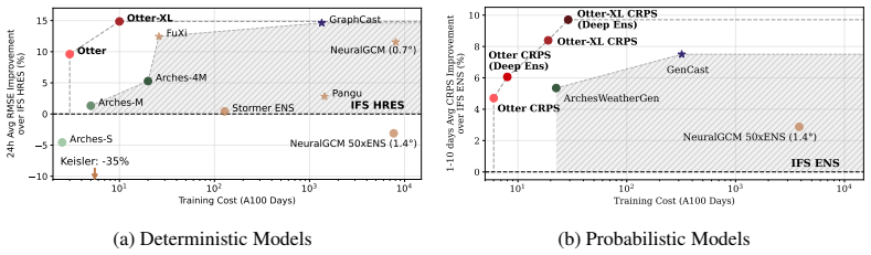
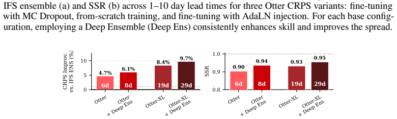
Otter Weather is a highly efficient spatiotemporal forecasting model that advances the skill-compute Pareto frontier. The deterministic version outperforms the best NWP baseline by 9.6 percent at 24-hour lead time while requiring fewer than 3.5 A100-days for training. It delivers a 2x efficiency gain over lightweight AI models and a 100-fold reduction relative to resource-intensive frontier architectures. Scaling to Otter-XL with CRPS training produces a 9.7 percent CRPS improvement over the IFS ENS baseline and outperforms GenCast by over 2 percent while using an order of magnitude less compute. The same model applied out-of-the-box to a complex acoustic scattering PDE task outperforms a st
What carries the argument
The Otter family of spatiotemporal forecasting models, which advance the skill-compute Pareto frontier through efficiency-focused design for weather prediction.
If this is right
- High-performance medium-range forecasts become feasible for groups with limited compute resources.
- Model development cycles for weather prediction shorten because training budgets drop by one to two orders of magnitude.
- Probabilistic forecasting skill improves at comparable compute budgets when models are trained directly with CRPS.
- The same efficiency-oriented design transfers to other scientific spatiotemporal tasks such as PDE modeling.
Where Pith is reading between the lines
- If the reported efficiency scales with resolution, ensembles of Otter models could run on modest hardware for operational use.
- The out-of-distribution success on an acoustic scattering task suggests the architecture may apply to other physical simulation domains without domain-specific redesign.
- Real-world deployment would still require separate verification that reanalysis skill carries over to live data streams and model drift.
Load-bearing premise
That performance measured on ERA5 reanalysis at 1.5 degree resolution with standard WeatherBench protocols will translate to operational forecasting skill.
What would settle it
Evaluating Otter forecasts on live operational weather observations over multiple seasons and comparing accuracy and reliability directly against current NWP systems.
Figures
read the original abstract
State-of-the-art medium-range AI weather models can outperform traditional Numerical Weather Prediction (NWP) but require massive training budgets. This restricts usage for under-resourced groups and severely limits fast model iteration. Here we develop Otter Weather, a highly efficient spatiotemporal forecasting model designed to democratise high-performance weather prediction with AI. Evaluated on ERA5 reanalysis data at 1.5{\deg} resolution using standard WeatherBench protocols, the Otter family significantly advances the skill-compute Pareto frontier. The deterministic version outperforms the best NWP baseline by 9.6% at a 24-hour lead time while requiring fewer than 3.5 A100-days for training. It provides a 2x efficiency gain over lightweight AI models and a 100-fold reduction in compute compared to resource-intensive frontier architectures. We extend these efficiency gains into probabilistic forecasting by training via the Continuous Ranked Probability Score (CRPS). Scaling to a larger architecture, Otter-XL achieves a 9.7% CRPS improvement over the IFS ENS baseline. This yields an almost two-fold increase in predictive skill over comparable lightweight models at similar compute budgets. Otter-XL also outperforms frontier architectures like GenCast by over 2%, while using an order of magnitude less compute. Finally, Otter is applied out-of-the-box to a complex acoustic scattering PDE task where it outperforms a state-of-the-art foundation modelling approach, suggesting that the advances made here might apply across a range of scientific domains.
Editorial analysis
A structured set of objections, weighed in public.
Referee Report
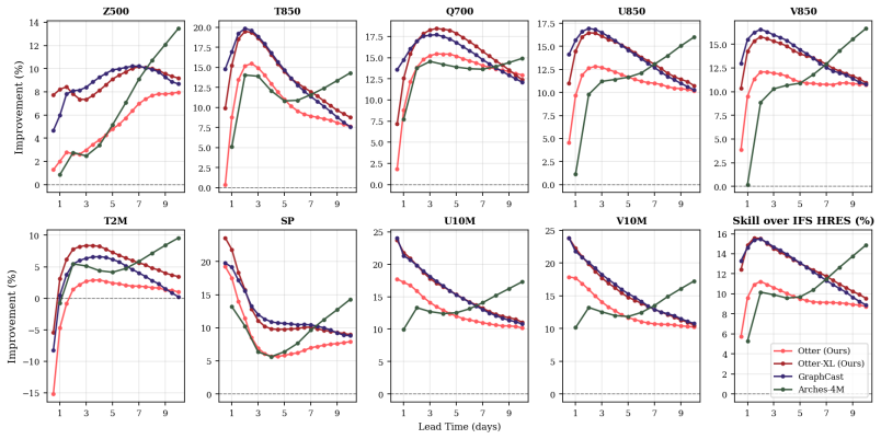
Summary. The manuscript introduces Otter Weather, a spatiotemporal AI model for medium-range weather forecasting. Evaluated on ERA5 reanalysis at 1.5° resolution with WeatherBench protocols, the deterministic version is claimed to outperform the best NWP baseline by 9.6% at 24-hour lead time while using fewer than 3.5 A100-days for training; a 2x efficiency gain over lightweight AI models and 100-fold reduction versus frontier models is reported. The work extends the approach to probabilistic forecasting via CRPS (Otter-XL achieving 9.7% improvement over IFS ENS), and demonstrates out-of-the-box application to an acoustic scattering PDE task.
Significance. If the performance and compute claims hold under full verification, the work would meaningfully advance the skill-compute Pareto frontier for AI weather models, lowering barriers for under-resourced groups and enabling faster iteration. The cross-domain PDE result provides additional evidence of broader applicability. The emphasis on reproducible low-compute training is a positive contribution if the end-to-end accounting is complete.
major comments (3)
- [§4] §4 (Results, deterministic model): The 9.6% outperformance claim at 24 h versus the best NWP baseline is load-bearing for the central efficiency claim but lacks explicit identification of the baseline (IFS deterministic vs. ensemble), the precise metric (RMSE vs. ACC), the variable set, and vertical levels; any mismatch with standard WeatherBench NWP comparisons would invalidate the percentage.
- [§5] §5 (Training and compute): The <3.5 A100-day training budget is central to the efficiency advantage but is presented without a full accounting of data staging, hyper-parameter sweeps, checkpointing, and validation passes; without this breakdown the quoted figure cannot be confirmed as the complete reproducible cost.
- [§3] §3 (Methods): No ablation studies, error bars, or sensitivity analyses on architecture or training choices are referenced in support of the reported gains; this omission prevents assessment of whether improvements are robust or attributable to post-hoc tuning.
minor comments (2)
- [Figure 2] Figure 2: Axis labels and legend entries for the Pareto frontier plot should explicitly state the exact metric and lead time used for each point to avoid ambiguity in cross-model comparisons.
- Notation: The definition of the spatiotemporal architecture (e.g., any custom convolution or attention blocks) should be given in a single equation block rather than scattered across text for clarity.
Simulated Author's Rebuttal
We thank the referee for their detailed and constructive comments on our manuscript. We address each major comment point by point below, providing clarifications and committing to revisions where appropriate to strengthen the paper.
read point-by-point responses
-
Referee: [§4] §4 (Results, deterministic model): The 9.6% outperformance claim at 24 h versus the best NWP baseline is load-bearing for the central efficiency claim but lacks explicit identification of the baseline (IFS deterministic vs. ensemble), the precise metric (RMSE vs. ACC), the variable set, and vertical levels; any mismatch with standard WeatherBench NWP comparisons would invalidate the percentage.
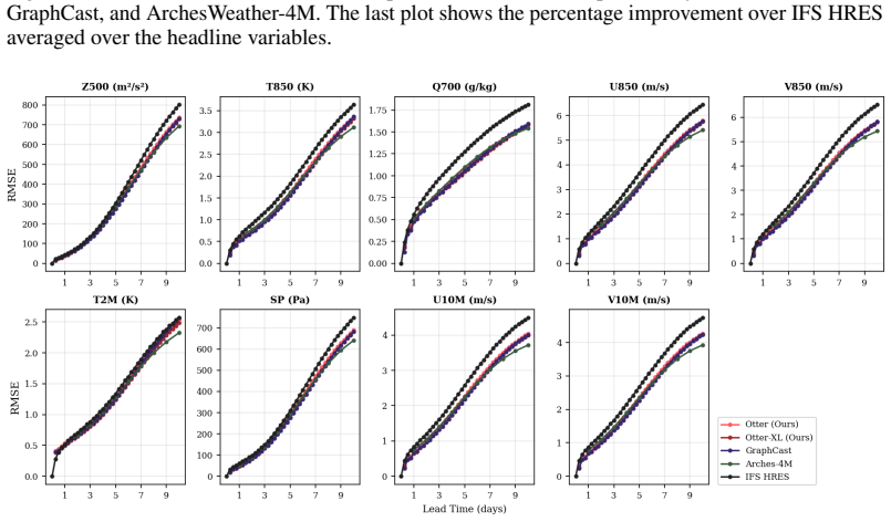
Authors: We appreciate the referee's attention to this detail. The 9.6% improvement is calculated as the relative reduction in RMSE for the deterministic Otter model compared to the IFS deterministic forecast (not ensemble) at 24-hour lead time, using the standard set of WeatherBench variables (2m temperature, 10m wind components, geopotential, specific humidity, etc.) at 1.5° resolution across all vertical levels where applicable. This aligns with WeatherBench protocols. To eliminate any potential for misinterpretation, we will revise §4 to explicitly state these parameters and include a supplementary table detailing the comparison. revision: yes
-
Referee: [§5] §5 (Training and compute): The <3.5 A100-day training budget is central to the efficiency advantage but is presented without a full accounting of data staging, hyper-parameter sweeps, checkpointing, and validation passes; without this breakdown the quoted figure cannot be confirmed as the complete reproducible cost.
Authors: The reported figure of fewer than 3.5 A100-days corresponds to the compute required for training the final Otter model after architecture selection. We recognize that a transparent end-to-end accounting is essential. In the revised manuscript, we will provide a comprehensive breakdown in §5, including estimates for data preparation, hyperparameter exploration (noting that sweeps were limited), checkpointing, and validation, to allow full verification of the total cost. revision: yes
-
Referee: [§3] §3 (Methods): No ablation studies, error bars, or sensitivity analyses on architecture or training choices are referenced in support of the reported gains; this omission prevents assessment of whether improvements are robust or attributable to post-hoc tuning.
Authors: We agree that ablations and sensitivity analyses would strengthen the claims. Although the primary results show consistent outperformance across multiple lead times and variables, we will incorporate additional analyses in the revised version, including sensitivity to key architectural choices (e.g., spatiotemporal attention mechanisms) and training hyperparameters, along with error bars from repeated training runs with different seeds where computationally feasible. revision: yes
Circularity Check
No circularity; empirical results are direct comparisons to external baselines
full rationale
The paper reports an ML model's performance on ERA5 reanalysis at 1.5° using WeatherBench protocols, with gains stated as direct numerical comparisons to external NWP baselines (IFS deterministic and ENS). No equations, derivations, or first-principles claims appear in the abstract or description. Efficiency figures are presented as measured training budgets versus other published models, not as quantities fitted from or defined by the target metrics. No self-citations, ansatzes, or uniqueness theorems are invoked as load-bearing steps. The derivation chain is therefore self-contained empirical evaluation against independent external references.
Axiom & Free-Parameter Ledger
Reference graph
Works this paper leans on
-
[1]
Anna Allen, Stratis Markou, Will Tebbutt, Wessel P
URL https://arxiv.org/ abs/2506.10772. Anna Allen, Stratis Markou, Will Tebbutt, Wessel P. Bruinsma, Tom R. Andersson, Michael Herzog, Nicholas D. Lane, Matthew Chantry, J. Scott Hosking, and Richard E. Turner. End-to-end data- driven weather prediction.Nature,
-
[2]
URL https: //www.nature.com/articles/s41586-025-08897-0
doi: 10.1038/s41586-025-08897-0. URL https: //www.nature.com/articles/s41586-025-08897-0. Zied Ben Bouallegue, Mihai Alexe, Matthew Chantry, Mariana Clare, Jesper Dramsch, Simon Lang, Christian Lessig, Linus Magnusson, Ana Prieto Nemesio, Florian Pinault, Baudouin Raoult, and Steffen Tietsche. New ml model on ecmwf web charts,
-
[3]
AIFS Blog
URL https://www.ecmwf.int/ en/about/media-centre/aifs-blog/2023/new-ml-model-ecmwf-web-charts . AIFS Blog. Kaifeng Bi, Lingxi Xie, Hengheng Zhang, Xin Chen, Xiaotao Gu, and Qi Tian. Pangu-weather: A 3d high-resolution model for fast and accurate global weather forecast,
2023
-
[4]
URL https: //arxiv.org/abs/2211.02556. Cristian Bodnar, Wessel P. Bruinsma, Ana Lucic, Megan Stanley, Anna Allen, Johannes Brandstetter, Patrick Garvan, Maik Riechert, Jonathan A. Weyn, Haiyu Dong, Jayesh K. Gupta, Kit Thambirat- nam, Alexander T. Archibald, Chun-Chieh Wu, Elizabeth Heider, Max Welling, Richard E. Turner, and Paris Perdikaris. A foundatio...
-
[5]
doi: 10.1038/s41586-025-09005-y
ISSN 1476-4687. doi: 10.1038/s41586-025-09005-y. URL https://doi.org/10.1038/s41586-025-09005-y . Boris Bonev, Thorsten Kurth, Ankur Mahesh, Mauro Bisson, Jean Kossaifi, Karthik Kashinath, Anima Anandkumar, William D. Collins, Michael S. Pritchard, and Alexander Keller. Fourcastnet 3: A geometric approach to probabilistic machine-learning weather forecast...
-
[6]
Salva Rühling Cachay, Miika Aittala, Hailey James, and Rose Yu
URLhttps://arxiv.org/abs/2507.12144. Salva Rühling Cachay, Miika Aittala, Hailey James, and Rose Yu. Elucidated rolling diffusion models for probabilistic forecasting of complex dynamics. InNeurIPS 2025,
arXiv 2025
-
[7]
Salva Ruhling Cachay, Duncan Watson-Parris, and Rose Yu
URL https: //arxiv.org/abs/2506.20024. Salva Ruhling Cachay, Duncan Watson-Parris, and Rose Yu. U-cast: A surprisingly simple and efficient frontier probabilistic ai weather forecaster.arXiv preprint arXiv:2604.09041,
-
[8]
Cristiana Diaconu, Miles Cranmer, Richard E
URLhttps://arxiv.org/abs/2412.12971. Cristiana Diaconu, Miles Cranmer, Richard E. Turner, Tanya Marwah, and Payel Mukhopadhyay. Probabilistic retrofitting of learned simulators,
-
[9]
URL https://arxiv. org/abs/1802.10026. Tilmann Gneiting and Adrian E. Raftery. Strictly proper scoring rules, prediction, and es- timation.Journal of the American Statistical Association, 102(477):359–378,
-
[10]
doi: 10.1198/016214506000001437. Ali Hassani, Steven Walton, Jiachen Li, Shen Li, and Humphrey Shi. Neighborhood attention transformer,
-
[11]
12 Kaiming He, Xinlei Chen, Saining Xie, Yanghao Li, Piotr Dollár, and Ross Girshick
URLhttps://arxiv.org/abs/2204.07143. 12 Kaiming He, Xinlei Chen, Saining Xie, Yanghao Li, Piotr Dollár, and Ross Girshick. Masked autoencoders are scalable vision learners,
-
[12]
URLhttps://arxiv.org/abs/2111.06377. Hans Hersbach, Bill Bell, Paul Berrisford, Gionata Biavati, András Horányi, Joaquín Muñoz Sabater, Julien Nicolas, Carole Peubey, Raluca Radu, Iryna Rozum, Dinand Schepers, Adrian Simmons, Cornel Soci, Dick Dee, and Jean-Noël Thépaut. The ERA5 global reanalysis.Quarterly Journal of the Royal Meteorological Society, 146...
Pith/arXiv arXiv 1999
-
[13]
doi: https://doi.org/10.1002/qj.3803. Keller Jordan, Yuchen Jin, Vlado Boza, You Jiacheng, Franz Cesista, Laker Newhouse, and Jeremy Bernstein. Muon: An optimizer for hidden layers in neural networks. https://kellerjordan. github.io/posts/muon/,
-
[14]
Ryan Keisler
Accessed: 2026-02-03. Ryan Keisler. Forecasting global weather with graph neural networks,
2026
-
[15]
URL https://arxiv. org/abs/2202.07575. Dmitrii Kochkov, J. Yuval, I. Langmore, P. Norgaard, J. Smith, G. Mooers, M. K. Klöwer, et al. Neural general circulation models for weather and climate.Nature, 632(8027):1060– 1066,
-
[16]
URL https://www.nature.com/articles/ s41586-024-07744-y
doi: 10.1038/s41586-024-07744-y. URL https://www.nature.com/articles/ s41586-024-07744-y. Balaji Lakshminarayanan, Alexander Pritzel, and Charles Blundell. Simple and scalable predictive uncertainty estimation using deep ensembles,
-
[17]
URLhttps://arxiv.org/abs/2212.12794. Simon Lang, Mihai Alexe, Matthew Chantry, Jesper Dramsch, Florian Pinault, Baudouin Raoult, Mariana C. A. Clare, Christian Lessig, Michael Maier-Gerber, Linus Magnusson, Zied Ben Bouallègue, Ana Prieto Nemesio, Peter D. Dueben, Andrew Brown, Florian Pappenberger, and Florence Rabier. Aifs – ecmwf’s data-driven forecast...
-
[18]
URL https://arxiv. org/abs/2406.01465. Simon Lang, Mihai Alexe, Matthew Chantry, Mariana Pinheiro, Peter Dueben, and Tim Palmer. Aifs-crps: Ensemble forecasting using a model trained with a loss function based on the continuous ranked probability score.npj Artificial Intelligence, 2(1),
-
[19]
doi: 10.1038/s44260-026-00045-z. Fanny Lehmann, Firat Ozdemir, Benedikt Soja, Torsten Hoefler, Siddhartha Mishra, and Sebastian Schemm. Finetuning a weather foundation model with lightweight decoders for unseen physical processes,
-
[20]
URLhttps://arxiv.org/abs/2506.19088. Jingyuan Liu, Jianlin Su, Xingcheng Yao, Zhejun Jiang, Guokun Lai, Yulun Du, Yidao Qin, Weixin Xu, Enzhe Lu, Junjie Yan, et al. Muon is scalable for llm training.arXiv preprint arXiv:2502.16982,
-
[21]
Ilya Loshchilov and Frank Hutter
URL https://arxiv.org/abs/2103.14030. Ilya Loshchilov and Frank Hutter. Fixing weight decay regularization in adam.CoRR, abs/1711.05101,
-
[22]
URLhttp://arxiv.org/abs/1711.05101. Ankur Mahesh, William Collins, Boris Bonev, Noah Brenowitz, Yair Cohen, Joshua Elms, Peter Harrington, Karthik Kashinath, Thorsten Kurth, Joshua North, Travis OBrien, Michael Pritchard, David Pruitt, Mark Risser, Shashank Subramanian, and Jared Willard. Huge ensembles part i: Design of ensemble weather forecasts using s...
-
[23]
URL https://arxiv.org/abs/2408.03100. 13 Michael McCabe, Payel Mukhopadhyay, Tanya Marwah, Bruno Regaldo-Saint Blancard, Francois Rozet, Cristiana Diaconu, Lucas Meyer, Kaze W. K. Wong, Hadi Sotoudeh, Alberto Bietti, Irina Espejo, Rio Fear, Siavash Golkar, Tom Hehir, Keiya Hirashima, Geraud Krawezik, Francois Lanusse, Rudy Morel, Ruben Ohana, Liam Parker,...
-
[24]
Tung Nguyen, Johannes Brandstetter, Ashish Kapoor, Jayesh K
URLhttps://arxiv.org/abs/2511.15684. Tung Nguyen, Johannes Brandstetter, Ashish Kapoor, Jayesh K. Gupta, and Aditya Grover. Climax: A foundation model for weather and climate,
-
[25]
URL https://arxiv.org/abs/2301.10343. Tung Nguyen, Rohan Shah, Hritik Bansal, Troy Arcomano, Romit Maulik, Veerabhadra Kotamarthi, Ian Foster, Sandeep Madireddy, and Aditya Grover. Scaling transformer neural networks for skillful and reliable medium-range weather forecasting,
-
[26]
Ruben Ohana, Michael McCabe, Lucas Meyer, Rudy Morel, Fruzsina J
URL https://arxiv.org/abs/ 2312.03876. Ruben Ohana, Michael McCabe, Lucas Meyer, Rudy Morel, Fruzsina J. Agocs, Miguel Beneitez, Mar- sha Berger, Blakesley Burkhart, Keaton Burns, Stuart B. Dalziel, Drummond B. Fielding, Daniel Fortunato, Jared A. Goldberg, Keiya Hirashima, Yan-Fei Jiang, Rich R. Kerswell, Suryanarayana Maddu, Jonah Miller, Payel Mukhopad...
-
[27]
URL https://arxiv.org/abs/2412.00568. Jaideep Pathak, Shashank Subramanian, Peter Harrington, Sanjeev Raja, Ashesh Chattopadhyay, Morteza Mardani, Thorsten Kurth, David Hall, Zongyi Li, Kamyar Azizzadenesheli, Pedram Hassanzadeh, Karthik Kashinath, and Animashree Anandkumar. Fourcastnet: A global data- driven high-resolution weather model using adaptive f...
-
[28]
Ilan Price, Alvaro Sanchez-Gonzalez, Ferran Alet, Tom R
URL https: //arxiv.org/abs/2202.11214. Ilan Price, Alvaro Sanchez-Gonzalez, Ferran Alet, Tom R. Andersson, Andrew El-Kadi, Dominic Masters, Timo Ewalds, Jacklynn Stott, Shakir Mohamed, Peter Battaglia, Remi Lam, and Matthew Willson. Gencast: Diffusion-based ensemble forecasting for medium-range weather,
-
[29]
Stephan Rasp, Stephan Hoyer, Aravind Merose, Johannes Langguth, Sebastian Deiser, et al
URL https://arxiv.org/abs/2312.15796. Stephan Rasp, Stephan Hoyer, Aravind Merose, Johannes Langguth, Sebastian Deiser, et al. Weath- erbench 2: A benchmark for the next generation of data-driven global weather models.arXiv preprint arXiv:2308.15560 (Also published in Journal of Advances in Modeling Earth Systems), 2023/2024. doi: 10.1029/2023MS004019. Ma...
-
[30]
URL https://arxiv.org/abs/2310.06743. Noam Shazeer. Glu variants improve transformer,
-
[31]
URL https://arxiv.org/abs/2002. 05202. Noam Shazeer, Azalia Mirhoseini, Krzysztof Maziarz, Andy Davis, Quoc Le, Geoffrey Hinton, and Jeff Dean. Outrageously large neural networks: The sparsely-gated mixture-of-experts layer,
2002
-
[32]
Jianlin Su, Yu Lu, Shengfeng Pan, Ahmed Murtadha, Bo Wen, and Yunfeng Liu
URLhttps://arxiv.org/abs/1701.06538. Jianlin Su, Yu Lu, Shengfeng Pan, Ahmed Murtadha, Bo Wen, and Yunfeng Liu. Roformer: Enhanced transformer with rotary position embedding,
-
[33]
URL https://arxiv.org/abs/ 2104.09864. Christopher Subich. Efficient fine-tuning of 37-level graphcast with the canadian global deterministic analysis.Artificial Intelligence for the Earth Systems, 4(3), July
-
[34]
ISSN 2769-7525. doi: 10.1175/aies-d-24-0101.1. URLhttp://dx.doi.org/10.1175/AIES-D-24-0101.1. Xiuyu Sun, Xiaohui Zhong, Xiaoze Xu, Yuanqing Huang, Hao Li, J. David Neelin, Deliang Chen, Jie Feng, Wei Han, Libo Wu, and Yuan Qi. Fuxi weather: A data-to-forecast machine learning system for global weather,
-
[35]
Defa Zhu, Hongzhi Huang, Zihao Huang, Yutao Zeng, Yunyao Mao, Banggu Wu, Qiyang Min, and Xun Zhou
URLhttps://arxiv.org/abs/2408.05472. Defa Zhu, Hongzhi Huang, Zihao Huang, Yutao Zeng, Yunyao Mao, Banggu Wu, Qiyang Min, and Xun Zhou. Hyper-connections,
-
[36]
URLhttps://arxiv.org/abs/2409.19606. 14 A Summary Table of Related Work We provide a comparative summary of deterministic weather models in table
-
[37]
Otter-XL closely approaches the performance of the best high-resolution model (GraphCast) despite using two orders of magnitude less compute
Despite operating with the lowest compute budget, Otter Weather achieves superior performance in the medium-resolution category and remains competitive with state-of-the-art models in the high-resolution regime. Otter-XL closely approaches the performance of the best high-resolution model (GraphCast) despite using two orders of magnitude less compute. Tab...
2024
-
[38]
constant-width
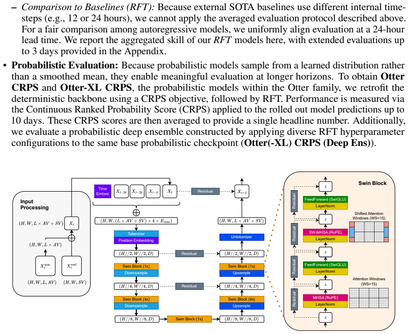
For every spatial location (h, w), we generate a dense feature vector containing all harmonic terms for degrees 0≤ℓ≤L max and orders −ℓ≤m≤ℓ . This results in (Lmax + 1)2 = 441 unique geometric features per pixel. These raw harmonic features are cached and passed through a learnable linear projection to match the token dimensionDbefore being added to the i...
2023
-
[39]
The downsampling operations reduce the spatial resolution by a factor of 2 at each stage (via 2×2 strided convolution) while maintaining the channel dimension constant at D
blocks. The downsampling operations reduce the spatial resolution by a factor of 2 at each stage (via 2×2 strided convolution) while maintaining the channel dimension constant at D. The skip connections use complex fusion (concatenation followed by a1×1convolution) rather than simple summation. B.2.4 Swin Transformer Block and Feed-Forward Network The fun...
2021
-
[40]
The aggregated loss sums over all target variables and pressure levelsv, averaging over lead timest= 1,
Mathematically, we can express the loss computed per variable v and at lead timetas: Lt v = vuut 1 HW HX i=1 WX j=1 w(ϕi), ˆX t i,j,v −X t i,j,v 2 (3) where w(ϕi) = cosϕ i 1 H PH k=1 cosϕ k downweights grid cells toward the poles, and ϕi is the latitude of row i over a uniform H×W grid. The aggregated loss sums over all target variables and pressure level...
2024
-
[41]
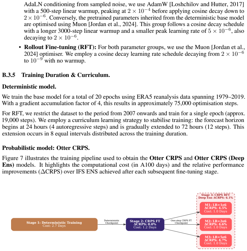
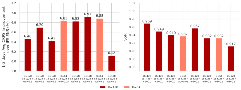
To form a deep ensemble, the pipeline branches to train three independent models for the equivalent of 1-A100 days each, using varied learning rates (10−6, 2×10 −6, and 5×10 −6)
In the final Rollout Fine-Tuning (RFT) phase (Stage 3), we restrict the dataset to the 2007–2019 period and apply the exact same curriculum learning strategy utilised for the deterministic model. To form a deep ensemble, the pipeline branches to train three independent models for the equivalent of 1-A100 days each, using varied learning rates (10−6, 2×10 ...
2007
-
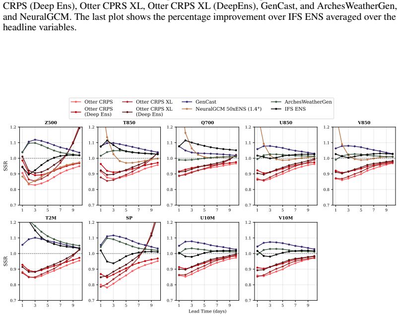
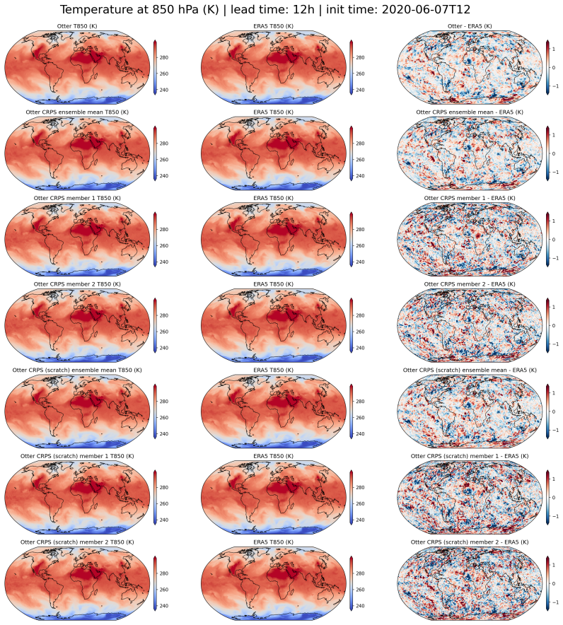
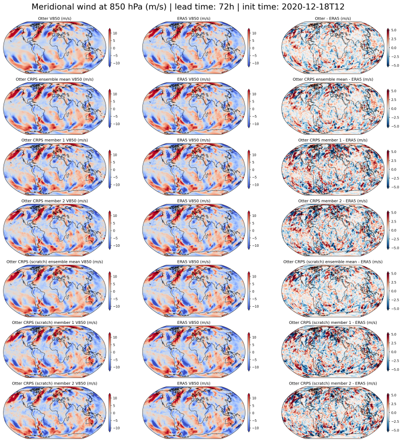
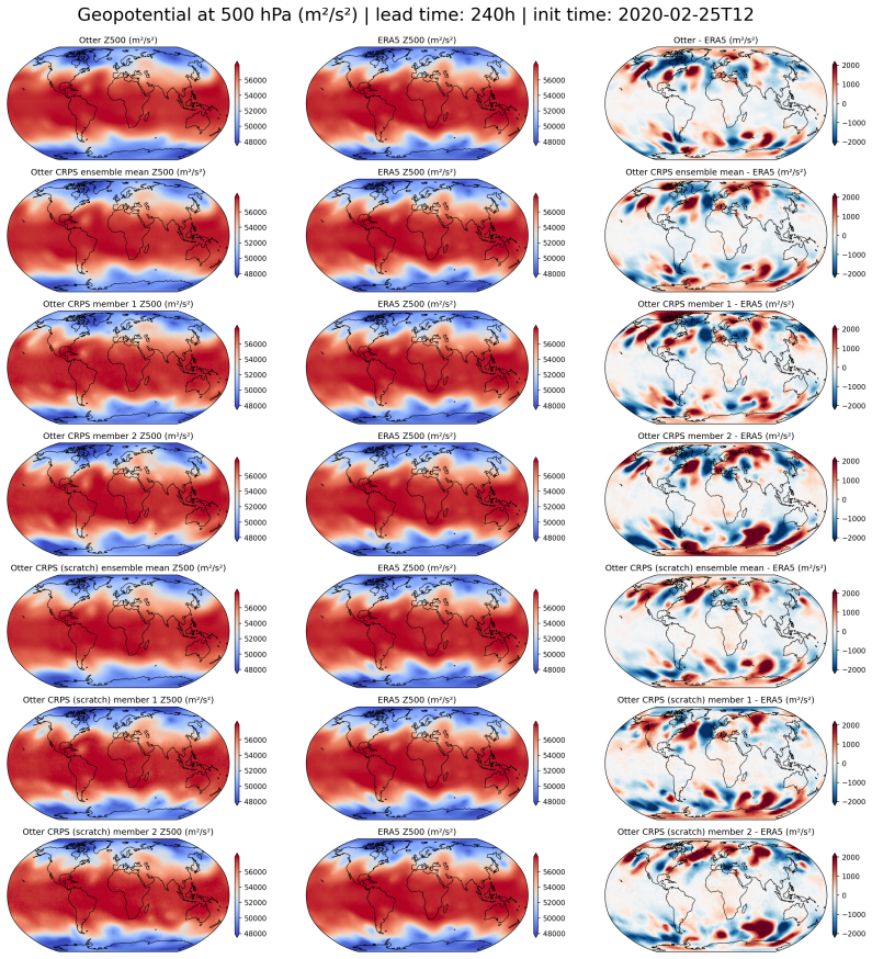
[42]
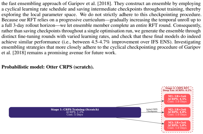
Probabilistic model: Otter CRPS (scratch)
remains a promising avenue for future work. Probabilistic model: Otter CRPS (scratch). Stage 2: CRPS RFT Deep Ens ΔCRPS: 6.2% Stage 1: CRPS Training (Scratch) ΔCRPS: 1.2% Cost: 5 Days M1: LR=1e6 ΔCRPS: 4.5% Cost: 1.0 Days M2: LR=2e6 ΔCRPS: 4.8% Cost: 1.0 Days Initial CRPS Checkpoint M3: LR=5e6 ΔCRPS: 5.0% Cost: 1.0 Days Figure 8: Overview of the training ...
1979
-
[43]
Stage 2 (CRPS fine-tuning) is executed for 5 epochs on the 1979–2019 ERA5 dataset. To obtain a single base model, we perform Rollout Fine-Tuning (RFT) for a single epoch on the 2007–2019 ERA5 data, employing the same curriculum learning strategy used for the deterministic model. To construct a deep ensemble version of the AdaLN model, we then independentl...
1979
-
[44]
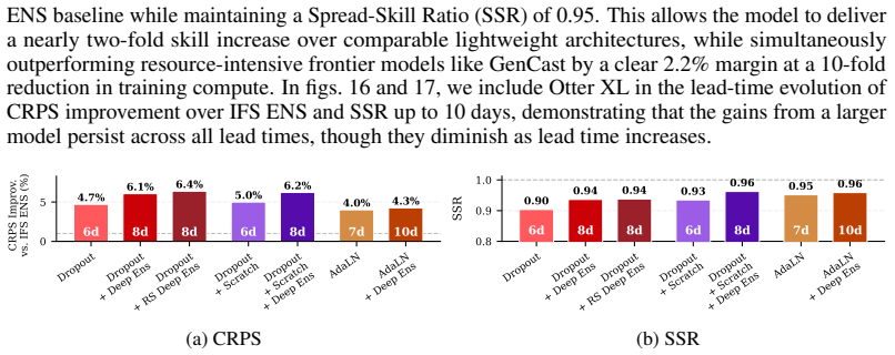
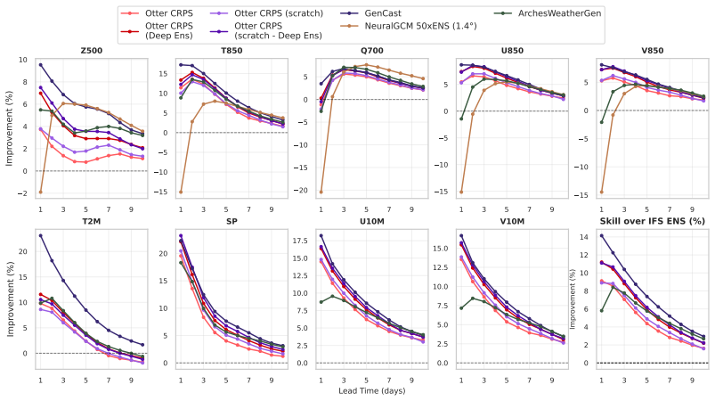
These lead to the following main observations: • Benefits of Deep Ensembling:Deep ensembling yields a consistent performance boost for the Otter CRPS models across all evaluated atmospheric variables. These gains are achieved at a minimal computational cost—in our case, the ensemble members were gen- erated by varying the learning rate during a standard h...
2025
-
[45]
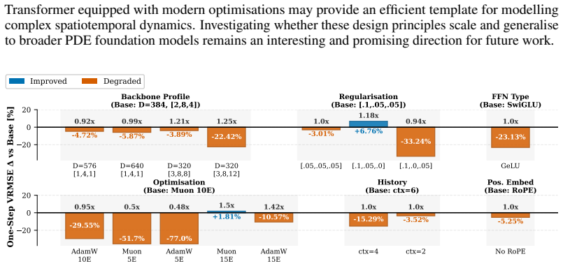
D.2 Base Deterministic Configuration
we use the following definition for the VRMSE: VRMSE(u, v) = s ⟨(u−v) 2⟩ ⟨(u− ⟨u⟩) 2⟩+ϵ ,(6) where⟨·⟩denotes the spatial mean operator and we addϵ= 10 −6 for numerical stability. D.2 Base Deterministic Configuration. The base configuration for PDE task is: •Embedding Dimension:D= 384; •Depth Profile (U-Net):[2,8,4]blocks per stage; •Attention Heads:16; •F...
2025
-
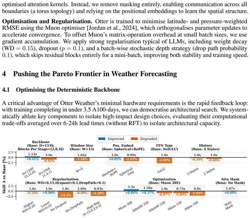
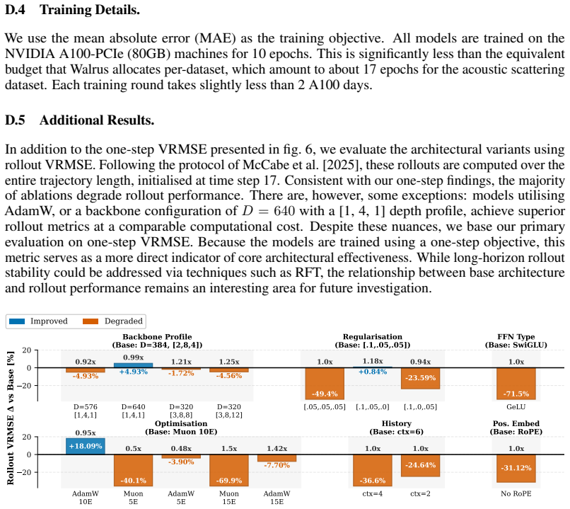
[46]
Consistent with our one-step findings, the majority of ablations degrade rollout performance. There are, however, some exceptions: models utilising AdamW, or a backbone configuration of D= 640 with a [1, 4, 1] depth profile, achieve superior rollout metrics at a comparable computational cost. Despite these nuances, we base our primary evaluation on one-st...
2025
discussion (0)
Sign in with ORCID, Apple, or X to comment. Anyone can read and Pith papers without signing in.