REVIEW 2 major objections 5 minor 34 references
Fast LiDAR Data Generation with Rectified Flows
T0 review · 2 major / 5 minor · reviewed 2026-08-11 · deepseek-v4-flash
Pith's one-line read This paper claims that rectified flows with reflow and timestep distillation let LiDAR range-reflectance generation keep fidelity at 1-4 sampling steps, matching or beating diffusion baselines at a fraction of the compute.
desk verdict R2Flow brings rectified flows to LiDAR generation with real few-step speed gains, but the 'outperforms' claim outruns the table and the raydrop-straightness question is honestly flagged but unresolved. read the letter →
The pith
A machine-rendered reading of the paper's core claim, the machinery that carries it, and where it could break.
The reading
What carries the argument
Rectified flow with reflow and timestep distillation: the model learns a velocity field $v_\theta(x_t,t)$ by matching the displacement $x_1-x_0$ along linear interpolation paths, then one reflow pass re-trains it on pairs $(x_1,x_0)$ generated by solving its own ODE, straightening trajectories, and a final timestep distillation trains only at the timesteps used by a fixed $k$-step Euler sampler. The velocity estimator is an hourglass transformer (HDiT-style) with circular sliding-window self-attention in the horizontal direction, landscape $1\times 4$ patches, beam-angle-conditioned rotary position embeddings, and a learned absolute positional bias; these modifications adapt a pixel-space transformer to panoramic LiDAR range and reflectance images. This machinery carries the paper's speed-quality argument: straight trajectories are what make few-step Euler sampling accurate, and the architecture is what keeps the pixel-space cost low enough to make iterative generation practical.
What would settle it
Measure the FRD gap between 2-RF + 4-TD at 4 steps and at 256 steps separately on range-image regions with and without raydrop pixels (pixels whose training target is $-1$); if the gap is concentrated in raydrop regions, or if training a raydrop-aware reflow loss (masking those pixels) does not reduce few-step FRD, the straightness assumption fails.
Extended reading notes
Core claim
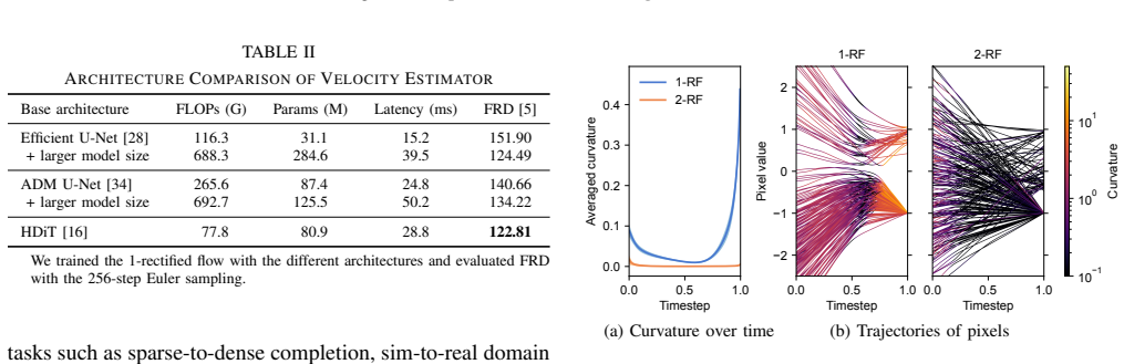
The paper's central claim is that LiDAR range-reflectance generation can shed the iterative cost of diffusion without losing fidelity by replacing stochastic curved SDE trajectories with deterministic straight ODE trajectories. Concretely, it shows that a 1-rectified-flow model (1-RF) trained with the conditional flow matching loss, after one reflow pass (2-RF) and timestep distillation (k-TD), produces samples whose quality degrades only mildly as the number of Euler steps drops from 256 to 1. The reported numbers are FRD 148.09 for 2-RF at 256 steps, 212.08 at 2 steps with 2-TD, and 187.10 at 4 steps with 4-TD, compared with R2DM's 2981.89 at 1 step and LiDM's 191.00 at 1 step, showing a flatter speed-quality curve than the diffusion baselines. At the high-step end, 1-RF achieves FRD 122.81 at 256 steps, competitive with R2DM's 154.11, so the rectified-flow formulation does not trade away top-end fidelity. The paper attributes the few-step robustness to trajectory straightening and to the proposed transformer architecture, which uses circular sliding-window attention, landscape patches, beam-angle-conditioned rotary embeddings, and an absolute positional embedding to keep azimuth alignment.
Load-bearing premise
The few-step advantage rests on the assumption that after reflow and timestep distillation the learned trajectories are straight enough for Euler sampling to stay accurate, and the paper itself notes in Section V that raydrop pixels drifting toward $-1$ may hinder straight-flow training; if those pixels keep trajectories curved, the 1-4 step gains would shrink.
Editorial extensions
If this is right
- If the central claim holds, LiDAR generative priors can run in a handful of network calls, making them usable in onboard robotics loops for sparse-to-dense completion or anomaly detection rather than offline only.
- The flat FRD-versus-NFE curve implies that a single trained model can be traded between quality and latency by choosing the number of steps at inference, without retraining.
- The inversion capability, demonstrated by scene interpolation, becomes a practical tool for LiDAR scene manipulation because the ODE can be run backward in few steps.
- Diffusion-based LiDAR generators should be revisited: the same evaluation protocol now shows rectified flows matching or beating DDPM and SMLD baselines at both high and low step counts.
- The architecture results indicate that pixel-space generation with transformers is competitive with latent-space approaches, so blur introduced by autoencoder decoding can be avoided.
Reading between the lines
- A testable extension the authors leave implicit: masking or reweighting the flow-matching loss at raydrop pixels (those flowing toward $-1$) before reflow could straighten the remaining curved trajectories and push the 1-2 step scores even closer to the 256-step scores.
- Because the 2-RF quality ceiling is set by the parent 1-RF, any gain in the 1-RF model (better architecture, more data, better raydrop handling) should propagate directly to the few-step distilled models, so architecture work and distillation work compound.
- The same straightening recipe should transfer to other range-sensor modalities (radar, sonar, depth cameras) that share the raydrop and missing-measurement phenomenon, since the paper's data representation only assumes a spherical range-reflectance image.
- If latency rather than FLOPs is the binding constraint in robotics, the paper's comparison suggests that step count, not parameter count, is the right optimization target for LiDAR generative models.
Signed reviews
Editorial analysis
A structured set of objections, weighed in public.
Referee Report
Summary. This paper presents R2Flow, a generative model for LiDAR range and reflectance images based on rectified flows. The authors train a 1-rectified flow (1-RF) with conditional flow matching, straighten it via reflow to obtain 2-RF, and then apply timestep distillation to produce few-step models (1-TD, 2-TD, 4-TD). They also introduce a pixel-space hourglass Vision Transformer architecture with circular sliding-window attention and landscape-shaped patches. On unconditional generation with the KITTI-360 dataset, R2Flow shows a better FRD-versus-NFE tradeoff than the tested GAN and diffusion baselines, with notably lower FRD at 1-4 function evaluations, while at 256 NFE it is competitive with but not uniformly better than R2DM on all metrics.
Significance. If the results are reproducible, the paper offers a practical speed-quality improvement for LiDAR generation, a domain where diffusion sampling cost is a practical barrier. The application of rectified flows is well grounded, the code and pretrained weights are provided, and the architecture ablation (Table II) supports the design choices in terms of FRD. The main contributions are the engineering of rectified-flow training for LiDAR data and an efficient Transformer backbone. However, the headline claim of outperforming state of the art for both large and small numbers of steps is stronger than the evidence, and the paper does not resolve the acknowledged difficulty of raydrop pixels in learning straight trajectories, which is exactly where the few-step promise is most at risk.
major comments (2)
- [Section I and Table I] The introduction states that 'our approach outperforms the state-of-the-art results for both large and small numbers of steps,' but Table I does not support the 'large steps' part. At 256 NFE, R2Flow 1-RF is worse than R2DM on FRID (4.18 vs 3.70), FPD (9.32 vs 3.79), FPVD (16.51 vs 10.90), and FSVD (15.07 vs 9.11), and 2-RF is worse on FRD, FRID, FPD, FPVD, and FSVD. The defensible conclusion is that R2Flow offers a better speed-quality tradeoff, not a categorical improvement at high step counts.
- [Section V and Figure 8] The central claim of the paper is that reflow and timestep distillation make trajectories straight enough for one to four Euler steps to preserve LiDAR fidelity. The authors themselves note in Section V that 'the raydrop pixels drifting toward a value of −1 may hinder the training of straight flows,' and Figure 8(b) associates the most curved trajectories with raydrop pixels. Yet no raydrop-specific evaluation is provided: there is no per-pixel curvature comparison between raydrop and non-raydrop pixels for 2-RF or the distilled models, no distributional comparison of raydrop masks in generated versus real scans, and no error bars or repeated-run statistics for any metric. Moreover, even the best few-step result, 2-RF+4-TD, has FRD 187.10, well above the 256-step 1-RF score of 122.81, so 'high-fidelity' few-step generation needs quantitative qualification. Without these analyses, the few-step advantage—the paper's main selling point—remains insufficiently supported for the raydrop component of LiDAR data.
minor comments (5)
- [Table I] The meaning of the 'Output' column is unclear from the table as presented; please clarify whether it indicates the modalities generated (range only, reflectance only, or both) and how each baseline is configured.
- [Table II] Table II reports only FRD for the architecture comparison; reporting a subset of the other metrics from Table I would strengthen the claim that the HDiT-based architecture is better overall, not merely on FRD.
- [Section IV-A] The paper does not explain why RangeLDM [8], which is discussed in the related work, is omitted from the experimental comparison; a sentence clarifying availability or scope would be helpful.
- [Figure 8] The caption for Figure 8(b) would benefit from explicitly stating that the pixel value −1 at t = 1 corresponds to raydrop noise, and from quantifying how many of the top-200 curved trajectories are raydrop pixels.
- [General] There are minor typographical issues, such as the capitalization after 'Following prior work' in Section III-B and the phrase 'example trajectory' in Section III-A, which should be 'example trajectories'.
Circularity Check
No significant circularity: the method applies published rectified-flow objectives and is evaluated against real KITTI-360 data, not against its own training outputs.
full rationale
The paper's central claim is an empirical speed-quality tradeoff measured with FRD, FRID, FPD, FPVD, FSVD, JSD, and MMD against the real KITTI-360 dataset. The training losses are the standard conditional flow matching loss and pseudo-Huber loss from Liu et al. [12] and Lee et al. [13], i.e., external first-principles formulations, not results derived from the paper's own conclusions. The reflow and timestep distillation stages do train on samples produced by the parent 1-RF model, but the authors explicitly acknowledge this dependency: "the 2-RF scores were slightly lower, which is because the quality upper bound for 2-RF is limited by the parent model 1-RF rather than real data" (Sec. IV-B). This is a stated limitation of the training procedure, not a prediction disguised as a fit. No parameter is fitted to a subset and then reported as a prediction of a closely related quantity; the few-step models are evaluated on the same held-out real-data metrics as all baselines. The paper's self-citations ([2], [3], [4]) are used as baselines, implementation details (circular padding), or future-work suggestions, and none is load-bearing for the few-step advantage claim. The admitted raydrop-straightness issue in Sec. V is a correctness risk regarding the robustness of the central claim, but it does not make the derivation circular. Overall, the evaluation is externally anchored and the reasoning chain is not self-referential in a way that forces the reported results.
Assumptions & free parameters
free parameters (4)
- pseudo-Huber constant c =
0.00054 * sqrt(d)
- timestep sampling shape a =
4
- range normalization maximum x_max =
unspecified in paper
- patch size and sliding window shape =
patch 1x4, window 3x9
assumptions (5)
- standard math Learning v_theta by minimizing conditional flow matching L_CFM yields an ODE whose solutions transport p0 to p1.
- standard math The reflow procedure straightens trajectories, and timestep distillation preserves quality at few target steps.
- domain assumption Euler integration with 1 to 256 steps accurately approximates the learned ODE solution.
- domain assumption The equirectangular 64x1024 range and reflectance representation preserves the geometric information needed for downstream point cloud use.
- domain assumption The Frechet and JSD/MMD metrics used in Table I reflect meaningful distributional fidelity.
Cite this review
Pith. "Pith review of Fast LiDAR Data Generation with Rectified Flows." pith.science (2026). https://pith.science/paper/ROJT4W7T
@misc{pith2026241202241,
  author       = {Pith},
  title        = {Pith review of: Fast LiDAR Data Generation with Rectified Flows},
  year         = {2026},
  howpublished = {\url{https://pith.science/paper/ROJT4W7T}},
  note         = {Machine review of arXiv:2412.02241}
}
read the original abstract
Building LiDAR generative models holds promise as powerful data priors for restoration, scene manipulation, and scalable simulation in autonomous mobile robots. In recent years, approaches using diffusion models have emerged, significantly improving training stability and generation quality. Despite their success, diffusion models require numerous iterations of running neural networks to generate high-quality samples, making the increasing computational cost a potential barrier for robotics applications. To address this challenge, this paper presents R2Flow, a fast and high-fidelity generative model for LiDAR data. Our method is based on rectified flows that learn straight trajectories, simulating data generation with significantly fewer sampling steps compared to diffusion models. We also propose an efficient Transformer-based model architecture for processing the image representation of LiDAR range and reflectance measurements. Our experiments on unconditional LiDAR data generation using the KITTI-360 dataset demonstrate the effectiveness of our approach in terms of both efficiency and quality.
Figures


Figures from the paper (5 more)


Reference graph
Works this paper leans on
-
[1]
Deep generative modeling of LiDAR data,
L. Caccia, H. van Hoof, A. Courville, and J. Pineau, “Deep generative modeling of LiDAR data,” in Proceedings of the IEEE/RSJ Interna- 0.0 0.5 1.0 Timestep 0.0 0.1 0.2 0.3 0.4Averaged curvature 1-RF 2-RF 0.0 0.5 1.0 Timestep −2 −1 0 1 2 Pixel value 1-RF 0.0 0.5 1.0 Timestep 2-RF 10−1 100 101 Curvature (a) Curvature over time (b) Trajectories of pixels Fig...
work page 2019
-
[2]
Learning to drop points for Li- DAR scan synthesis,
K. Nakashima and R. Kurazume, “Learning to drop points for Li- DAR scan synthesis,” in Proceedings of the IEEE/RSJ International Conference on Intelligent Robots and Systems (IROS) , pp. 222–229, 2021
work page 2021
-
[3]
Generative range imaging for learning scene priors of 3D LiDAR data,
K. Nakashima, Y . Iwashita, and R. Kurazume, “Generative range imaging for learning scene priors of 3D LiDAR data,” in Proceedings of the IEEE/CVF Winter Conference on Applications of Computer Vision (WACV), pp. 1256–1266, 2023
work page 2023
-
[4]
LiDAR data synthesis with denois- ing diffusion probabilistic models,
K. Nakashima and R. Kurazume, “LiDAR data synthesis with denois- ing diffusion probabilistic models,” in Proceedings of the IEEE Inter- national Conference on Robotics and Automation (ICRA) , pp. 14724– 14731, 2024
work page 2024
-
[5]
Learning to generate realistic LiDAR point clouds,
V . Zyrianov, X. Zhu, and S. Wang, “Learning to generate realistic LiDAR point clouds,” in Proceedings of the European Conference on Computer Vision (ECCV) , pp. 17–35, 2022
work page 2022
-
[6]
Towards realistic scene generation with LiDAR diffusion models,
H. Ran, V . Guizilini, and Y . Wang, “Towards realistic scene generation with LiDAR diffusion models,” in Proceedings of the IEEE/CVF Conference on Computer Vision and Pattern Recognition (CVPR) , 2024
work page 2024
-
[7]
Learning compact representations for lidar completion and generation,
Y . Xiong, W.-C. Ma, J. Wang, and R. Urtasun, “Learning compact representations for lidar completion and generation,” in Proceedings of the IEEE/CVF Conference on Computer Vision and Pattern Recog- nition (CVPR), pp. 1074–1083, 2023
work page 2023
-
[8]
RangeLDM: Fast realistic LiDAR point cloud generation,
Q. Hu, Z. Zhang, and W. Hu, “RangeLDM: Fast realistic LiDAR point cloud generation,” in Proceedings of the European Conference on Computer Vision (ECCV) , p. 115–135, 2024
work page 2024
Show all 34 references
-
[9]
Deep gen- erative modelling: A comparative review of V AEs, GANs, normalizing flows, energy-based and autoregressive models,
S. Bond-Taylor, A. Leach, Y . Long, and C. G. Willcocks, “Deep gen- erative modelling: A comparative review of V AEs, GANs, normalizing flows, energy-based and autoregressive models,”IEEE Transactions on Pattern Analysis and Machine Intelligence (TPAMI) , vol. 44, no. 11, pp. ...
2022
-
[10]
Score-based generative modeling through stochastic differential equations,
Y . Song, J. Sohl-Dickstein, D. P. Kingma, A. Kumar, S. Ermon, and B. Poole, “Score-based generative modeling through stochastic differential equations,” in Proceedings of the International Conference on Learning Representations (ICLR) , 2021
2021
-
[11]
Scalable diffusion models with transform- ers,
W. Peebles and S. Xie, “Scalable diffusion models with transform- ers,” in Proceedings of the IEEE/CVF International Conference on Computer Vision (ICCV) , pp. 4195–4205, 2023
2023
-
[12]
Flow straight and fast: Learning to generate and transfer data with rectified flow,
X. Liu, C. Gong, and Q. Liu, “Flow straight and fast: Learning to generate and transfer data with rectified flow,” in Proceedings of the International Conference on Learning Representations (ICLR) , 2023
2023
-
[13]
Improving the training of rectified flows,
S. Lee, Z. Lin, and G. Fanti, “Improving the training of rectified flows,” in Advances in Neural Information Processing Systems (NeurIPS) , vol. 37, pp. 63082–63109, 2024
2024
-
[14]
Flow matching for generative modeling,
Y . Lipman, R. T. Q. Chen, H. Ben-Hamu, M. Nickel, and M. Le, “Flow matching for generative modeling,” in Proceedings of the International Conference on Learning Representations (ICLR) , 2023
2023
-
[15]
Improving and generalizing flow- based generative models with minibatch optimal transport,
A. Tong, K. FATRAS, N. Malkin, G. Huguet, Y . Zhang, J. Rector- Brooks, G. Wolf, and Y . Bengio, “Improving and generalizing flow- based generative models with minibatch optimal transport,” Transac- tions on Machine Learning Research (TMLR) , 2024
2024
-
[16]
Scalable high-resolution pixel-space image synthesis with hourglass diffusion transformers,
K. Crowson, S. A. Baumann, A. Birch, T. M. Abraham, D. Z. Kaplan, and E. Shippole, “Scalable high-resolution pixel-space image synthesis with hourglass diffusion transformers,” in Proceedings of the International Conference on Machine Learning (ICML) , 2024
2024
-
[17]
KITTI-360: A novel dataset and benchmarks for urban scene understanding in 2D and 3D,
Y . Liao, J. Xie, and A. Geiger, “KITTI-360: A novel dataset and benchmarks for urban scene understanding in 2D and 3D,” IEEE Transactions on Pattern Analysis and Machine Intelligence (TPAMI) , vol. 45, no. 3, pp. 3292–3310, 2022
2022
-
[18]
Auto-encoding variational bayes,
D. P. Kingma and M. Welling, “Auto-encoding variational bayes,” in Proceedings of the International Conference on Learning Representa- tions (ICLR), 2014
2014
-
[19]
Neural discrete representation learning,
A. Van Den Oord, O. Vinyals, et al., “Neural discrete representation learning,” in Advances in Neural Information Processing Systems (NeurIPS), vol. 30, 2017
2017
-
[20]
Generative adversarial nets,
I. Goodfellow, J. Pouget-Abadie, M. Mirza, B. Xu, D. Warde-Farley, S. Ozair, A. Courville, and Y . Bengio, “Generative adversarial nets,” in Advances in Neural Information Processing Systems (NeurIPS) , pp. 2672–2680, 2014
2014
-
[21]
Generative modeling by estimating gradients of the data distribution,
Y . Song and S. Ermon, “Generative modeling by estimating gradients of the data distribution,” inAdvances in Neural Information Processing Systems (NeurIPS), pp. 11895–11907, 2019
2019
-
[22]
Improved techniques for training score-based generative models,
Y . Song and S. Ermon, “Improved techniques for training score-based generative models,” in Advances in Neural Information Processing Systems (NeurIPS), vol. 33, pp. 12438–12448, 2020
2020
-
[23]
Denoising diffusion probabilistic models,
J. Ho, A. Jain, and P. Abbeel, “Denoising diffusion probabilistic models,” in Advances in Neural Information Processing Systems (NeurIPS), vol. 33, pp. 6840–6851, 2020
2020
-
[24]
Variational diffusion models,
D. Kingma, T. Salimans, B. Poole, and J. Ho, “Variational diffusion models,” in Advances in Neural Information Processing Systems (NeurIPS), vol. 34, pp. 21696–21707, 2021
2021
-
[25]
High-resolution image synthesis with latent diffusion models,
R. Rombach, A. Blattmann, D. Lorenz, P. Esser, and B. Ommer, “High-resolution image synthesis with latent diffusion models,” in Proceedings of the IEEE/CVF Conference on Computer Vision and Pattern Recognition (CVPR), pp. 10684–10695, 2022
2022
-
[26]
Neighborhood attention transformer,
A. Hassani, S. Walton, J. Li, S. Li, and H. Shi, “Neighborhood attention transformer,” in Proceedings of the IEEE/CVF Conference on Computer Vision and Pattern Recognition (CVPR), pp. 6185–6194, 2023
2023
-
[27]
An image is worth 16x16 words: Transformers for image recognition at scale,
A. Dosovitskiy, L. Beyer, A. Kolesnikov, D. Weissenborn, X. Zhai, T. Unterthiner, M. Dehghani, M. Minderer, G. Heigold, S. Gelly, J. Uszkoreit, and N. Houlsby, “An image is worth 16x16 words: Transformers for image recognition at scale,” in Proceedings of the International Con...
2021
-
[28]
Photorealistic text-to-image diffusion models with deep lan- guage understanding,
C. Saharia, W. Chan, S. Saxena, L. Li, J. Whang, E. L. Denton, K. Ghasemipour, R. Gontijo Lopes, B. Karagol Ayan, T. Salimans, et al. , “Photorealistic text-to-image diffusion models with deep lan- guage understanding,” in Advances in Neural Information Processing Systems (Neu...
2022
-
[29]
TULIP: Transformer for upsampling of LiDAR point clouds,
B. Yang, P. Pfreundschuh, R. Siegwart, M. Hutter, P. Moghadam, and V . Patil, “TULIP: Transformer for upsampling of LiDAR point clouds,” in Proceedings of the IEEE/CVF Conference on Computer Vision and Pattern Recognition (CVPR), pp. 15354–15364, 2024
2024
-
[30]
RoFormer: Enhanced transformer with rotary position embedding,
J. Su, Y . Lu, S. Pan, B. Wen, and Y . Liu, “RoFormer: Enhanced transformer with rotary position embedding,” arXiv:2104.09864, 2021
2021 arXiv
-
[31]
All are worth words: A ViT backbone for diffusion models,
F. Bao, S. Nie, K. Xue, Y . Cao, C. Li, H. Su, and J. Zhu, “All are worth words: A ViT backbone for diffusion models,” in Proceedings of the IEEE/CVF Conference on Computer Vision and Pattern Recognition (CVPR), pp. 22669–22679, 2023
2023
-
[32]
3D point cloud generative adversarial network based on tree structured graph convolutions,
D. W. Shu, S. W. Park, and J. Kwon, “3D point cloud generative adversarial network based on tree structured graph convolutions,” in Proceedings of the IEEE/CVF International Conference on Computer Vision (ICCV), pp. 3859–3868, 2019
2019
-
[33]
torchdiffeq,
R. T. Q. Chen, “torchdiffeq,” 2018
2018
-
[34]
Diffusion models beat gans on image synthesis,
P. Dhariwal and A. Nichol, “Diffusion models beat gans on image synthesis,” in Advances in Neural Information Processing Systems (NeurIPS), vol. 34, pp. 8780–8794, 2021
2021
Reviewed August 11, 2026 · model on record in the stance chip above.
Discussion (0). Continue with ORCID to comment.