REVIEW 3 major objections 5 minor 52 references
Grokking vs. Learning: Same Features, Different Encodings
T0 review · 3 major / 5 minor · reviewed 2026-08-09 · deepseek-v4-flash
Pith's one-line read The paper claims that grokking and ordinary steady training converge on the same features in modular addition and Ising-phase classification, but that steady training can encode those features far more efficiently—most strikingly in a…
desk verdict The compressive regime is a genuine new result, but the 'same features' headline overstates the paper's own Ising appendix. read the letter →
The pith
A machine-rendered reading of the paper's core claim, the machinery that carries it, and where it could break.
The reading
What carries the argument
Several objects carry the argument. Grokking is induced and controlled by a single dial: the multiplier $w_0$ applied to the initialization weights, which smoothly interpolates between steady learning and grokking. Features are read out by task-specific probes—pre-activation correlation coefficients against energy and magnetization for the Ising classifier, and the inverse participation ratio in the Fourier basis, $\mathrm{IPR}^{(k)} = \sum_{\nu} |\tilde{W}_{\nu k}|^4 / (\sum_{\nu} \tilde{W}_{\nu k}^2)^2$, for modular addition. Compressibility is quantified by pruning each layer's smallest weights by a fraction $p$, integrating the resulting accuracy curve $a(p)$, and setting $c = 1/(1-a)$; the compressive regime is the region where $c$ and end train loss trade off linearly. Finally, the trajectory analysis uses the Fisher information metric $g^{\mathrm{FIM}}_{ij}$ to define a step magnitude $|s|_{\mathrm{FIM}}$ and a cosine similarity $S_{C-\mathrm{FIM}}(s,s')$ between consecutive parameter-space steps, which reveal the straight-line grokking path.
What would settle it
A concrete check: apply a pruning rule that does not rank weights by magnitude within each layer—for instance, pruning by diagonal Fisher information—to the modular addition models in the compressive regime. If the 25x compression advantage disappears, or if a non-magnitude-pruned grokked model prunes as well as the steady one, then the claimed encoding-efficiency difference is a property of the magnitude-pruning metric rather than of the learned representations; alternatively, a synthetic task with two provably distinct solution families could test whether the feature probes ever miss a genuinely different strategy in one of the two training regimes.
Extended reading notes
Core claim
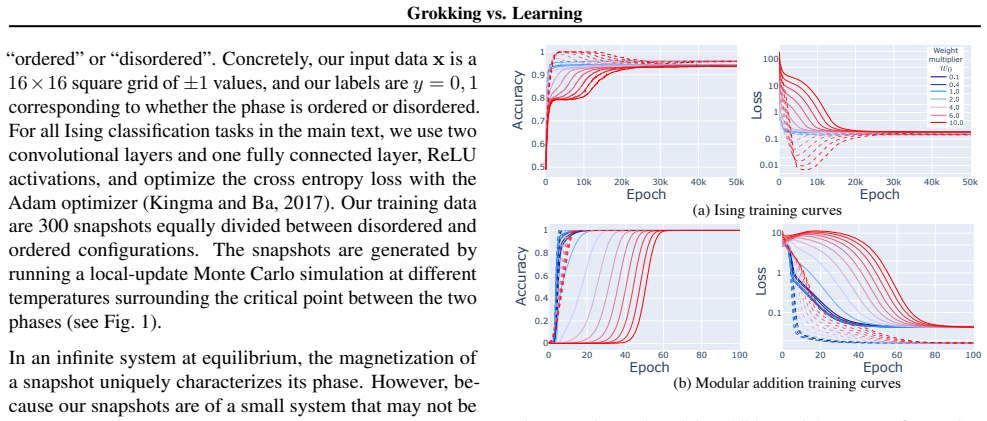
The central claim is that grokked and steadily trained models learn exactly the same dataset features, but the efficiency with which those features are encoded can differ by a large factor. The authors establish this by correlating final-layer pre-activations with the physically meaningful features in each task: energy and magnetization for the Ising CNN, and Fourier-basis localization (inverse participation ratio) for the modular addition MLP. They then introduce a compressibility measure based on the area under the magnitude-pruning curve and show that, in modular addition, models trained in a parameter range they call the compressive regime obey a linear trade-off between end train loss and compressibility, reaching compression factors of 25x the base model and 5x the best grokked compression. In the Ising task no compressive regime appears, which the authors take to show that the phenomenon is a distinct, parameter-dependent regime of steady learning rather than a generic feature of training. Dynamically, the paper reports that feature formation during the grokking plateau is task-dependent (visible in modular addition, absent in Ising), that compressibility peaks immediately after the plateau, and that the grokking trajectory follows an approximately straight line in model space as measured by a Fisher-information-based cosine similarity.
Load-bearing premise
The load-bearing assumption is that the hand-built interpretability scores—pre-activation correlation with energy and magnetization for Ising, Fourier-basis inverse participation ratio for modular addition—faithfully report the features the network actually uses, so that the 'same features' conclusion would fail if these probes miss the true computational strategy.
Editorial extensions
If this is right
- The practical upside of grokking is not that it discovers better features: at least in these tasks, steady training finds the same ones, and can find them in a more prunable form.
- In modular addition, initialization scale becomes a dial that trades final train loss against model size after pruning, so a practitioner can pick a point on that trade-off curve.
- The compressive regime is parameter-specific and can be switched off (e.g., by raising batch size), so compression advantages must be reported together with the training hyperparameters that produce them.
- Peak compressibility occurs just after the grokking plateau, and a transient compressibility spike appears even in runs without the compressive regime, so pruning dynamics and terminal compressibility are separate phenomena.
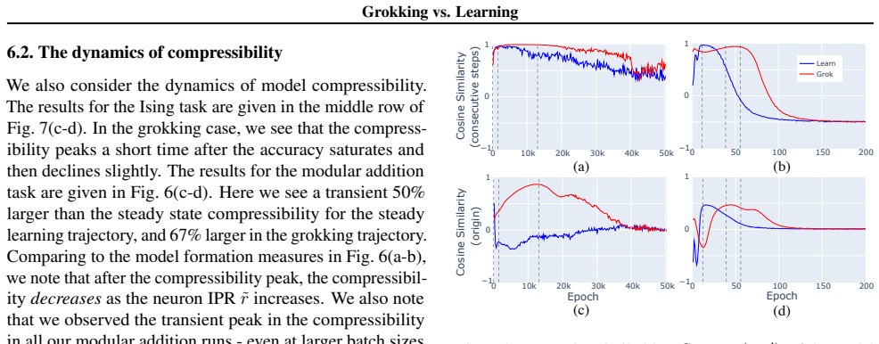
- Fisher-information-based trajectory measures give a task-general signature of grokking—nearly straight paths in model space—that does not depend on hand-built feature probes.
Reading between the lines
- If the same-features conclusion generalizes beyond toy tasks, then the main remaining reason to prefer grokking would be some other dynamic benefit, and the paper's own evidence would argue for eliminating grokking whenever possible—a claim the authors put forward as an open question.
- The linear loss–compressibility trade-off looks like a rate–distortion curve indexed by the initial weight scale; viewing it this way suggests the compressive regime might be generically predicted by an information-theoretic account of how initialization scale limits the model's effective capacity.
- The two-root signature in the gradient of the FIM step magnitude could be tested as a universal grokking detector on tasks where no interpretable 'progress measure' exists; if it marks the plateau start and end across many architectures, it would make hand-built probes unnecessary for detecting grokking.
- The reported absence of a correlation between compressibility and the local learning coefficient is surprising under the usual intuition that more degenerate models are more compressible, and could motivate a re-examination of what the local learning coefficient measures.
Editorial analysis
A structured set of objections, weighed in public.
Referee Report
Summary. The paper compares neural networks trained via grokking and via ordinary 'steady' learning on two controlled tasks: classifying phases of 2D Ising snapshots with a CNN, and modular addition with a one-hidden-layer MLP. The authors sweep only the initialization weight scale to interpolate between regimes, keeping architecture, data, and optimizer fixed. Their central claims are: (1) grokked and steadily trained models learn the same dataset features (energy/magnetization for Ising; Fourier modes for modular addition), (2) the encodings differ, most strikingly in a 'compressive regime' of steady training in modular addition where there is a linear trade-off between end train loss and compressibility, reaching roughly 25x compression of the base model under higher weight decay, (3) model development during the grokking plateau is task-dependent, with modular addition showing progress measures and Ising showing none, and (4) information-geometric measures based on the Fisher Information Metric show that grokking trajectories are approximately straight in model space. The paper includes per-seed data in appendices and provides code.
Significance. The compressive regime is the strongest contribution: it is a reproducible, controlled finding with potential practical value for model compression, and the claim is supported by per-seed plots and a check that increasing batch size removes the effect. The FIM-based trajectory analysis is a novel measurement tool that is general and, if validated, could be useful beyond these two tasks. The authors are to be credited for fixing architecture/data and varying only the initialization scale, for reporting per-seed distributions, and for releasing code. However, the headline 'same features' conclusion is currently overstated: the Ising claim is contradicted by the paper's own Appendix C, and the compressive-regime results in Appendix E show that the steady model's Fourier localization can break down, complicating the feature-identity statement. If the authors can resolve the Ising discrepancy and qualify the feature-identity claim, the paper would be a solid empirical contribution.
major comments (3)
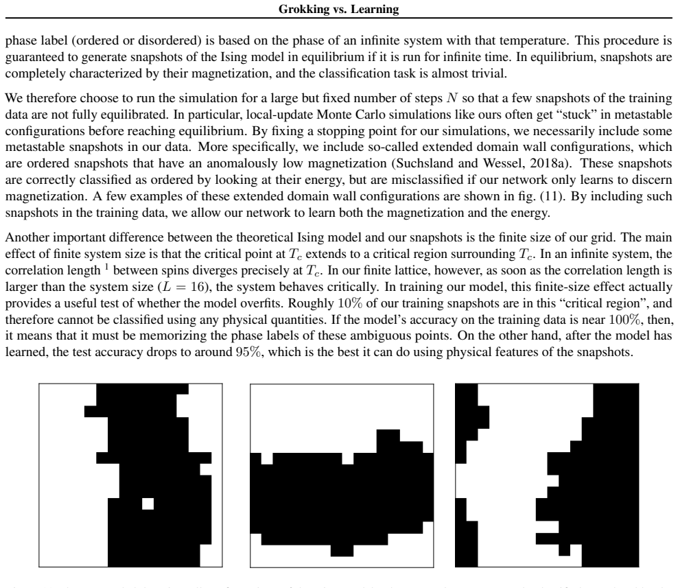
- [§4.1 and Appendix C] Section 4.1 states that 'every neuron in the final layer is either perfectly correlated or anti-correlated with the energy of the input' and that 'for every seed, in both learning and grokking, the energy has the highest correlation' with the majority of neurons in the second CNN and fully connected layer. Appendix C (Fig. 13 and surrounding text) reports the opposite: in the grokking regime, 'three of the seeds have significant deviation from perfect correlation with the energy, and instead correlate to the raw value of the magnetization,' and the caption says 'in some seeds learning the magnetization.' These statements cannot both be true. The same-features claim is the first headline conclusion, so the paper must quantify the per-seed/per-neuron deviations, report whether the three deviating seeds reach the same test accuracy as the others, and either restrict the conclusion to the majority of seeds or explain why magnetization-correlated neurons are consistent with 'learning the same feature.' The deliberate construction of the dataset to favor energy (§4.1) additionally means the near-universal energy correlation is partly a property of the task design.
- [§4.2, §5, Appendix D/E] The same-features conclusion is also in tension with the compressive regime. In §4.2, IPR localization is used as evidence that grokked and steadily trained models learn the same Fourier features (comparable mean IPRs of 0.43 and 0.53). Yet Appendix D reports that the compressive regime 'leads to an improvement in compressibility through a decrease in Fourier basis localization,' and Appendix E states that in the highly compressive regime 'the mean IPR falls by close to an order of magnitude, indicating that the model's Fourier representation is breaking down.' If IPR is a feature-identity measure, then a steady model in the compressive regime does not share the same localized Fourier features as a grokked model. The main text should state this caveat explicitly and clarify what 'same features' means for delocalized representations.
- [Abstract and §6.3] The abstract claims that 'models undergoing grokking follow a straight path in information space,' but the evidence in §6.3 is a peak cosine similarity that is near one only for the Ising grokking regime; for modular addition the peak is noticeably lower, and in all regimes the consecutive-step cosine similarity decays to near zero after learning. The straight-line statement should be restricted to the pre-/during-grokking phase and to the Ising task, or additional per-seed evidence should be provided showing straightness in modular addition grokking.
minor comments (5)
- [Figure 13 caption] The caption of Figure 13 says 'the dominant behaviour is still to learn the magnetization,' which contradicts the body text's claim that energy is the dominant feature; please correct the likely typo or reconcile the statement with §4.1.
- [§5 and Appendix E] The text alternates between the area-based compressibility c of Eq. (5) and the weight fraction needed to maintain 95% accuracy ('cut 95% of the weights'); the relationship between these two quantities should be stated explicitly so that '25x compression' is unambiguous.
- [Table 1] The Ising task uses weight decay 0.1 while modular addition uses 3e-5; because weight decay is the mechanism behind the straight-to-the-origin trajectory in §6.3, the large asymmetry between the two tasks should be discussed when comparing their dynamics.
- [Appendix F] The FIM is approximated by its diagonal, citing Amari et al. (2019), but no numerical check of the diagonal approximation is reported for these specific architectures; a brief validation would strengthen the FIM-based conclusions.
- [§2.2] The one-hot vector notation in §2.2 has typographical artifacts (e.g., '0 1, ...,1a, ...,0P'); please clean up the notation.
Circularity Check
No significant circularity: central claims are empirical measurements and parameter scans; self-cited FIM tools are measurement devices, not inputs.
full rationale
The paper is an empirical study, not a derivation, and I find no step in which a claimed result is identical to an input by construction. The same-features conclusions are supported by independently measured correlation coefficients (Section 4.1) and Fourier IPRs (Section 4.2), both computed on trained models; the design choice to favor energy is an input, but the equal-energy conclusion across grokking and steady training is not definitional. The compressive-regime result (Section 5) is a parameter scan: the weight multiplier w0 is varied, and end train loss and pruning-area compressibility are measured separately; the observed linear trade-off is an empirical curve, not a fitted constraint. The FIM trajectory measures (Section 6.3) are self-cited to Berman et al., but the FIM is a standard object and the cited works are used as a measurement toolkit, not to force the straight-line conclusion. I therefore score no circularity. I do flag one internal inconsistency that is a correctness concern rather than circularity: Appendix C (Fig. 13) reports that in the grokking Ising regime 'three of the seeds have significant deviation from perfect correlation with the energy, and instead correlate to the raw value of the magnetization,' which weakens the main-text claim in Section 4.1 that 'every neuron in the final layer is either perfectly correlated or anti-correlated with the energy.' This per-seed variability should be reconciled, but it does not make the conclusion an input of the analysis.
Assumptions & free parameters
free parameters (4)
- weight multiplier w0 =
swept; Ising 1-10, modular addition 0.1-100
- weight decay for high-compression runs =
3e-4 versus 3e-5
- FIM diagonal threshold =
0.1
- batch size =
64 main text, 200 control
assumptions (5)
- domain assumption Pre-activation correlation and Fourier IPR faithfully measure the features the network uses.
- ad hoc to paper Grokking is adequately defined by the 5% train and test accuracy margins in Definition 1.
- domain assumption The FIM diagonal approximation holds for these networks.
- domain assumption The two toy tasks are informative representatives of grokking behavior.
- domain assumption The Ising dataset design biases the model toward the energy feature.
Cite this review
Pith. "Pith review of Grokking vs. Learning: Same Features, Different Encodings." pith.science (2026). https://pith.science/paper/SGERGN6V
@misc{pith2026250201739,
  author       = {Pith},
  title        = {Pith review of: Grokking vs. Learning: Same Features, Different Encodings},
  year         = {2026},
  howpublished = {\url{https://pith.science/paper/SGERGN6V}},
  note         = {Machine review of arXiv:2502.01739}
}
read the original abstract
Grokking typically achieves similar loss to ordinary, "steady", learning. We ask whether these different learning paths - grokking versus ordinary training - lead to fundamental differences in the learned models. To do so we compare the features, compressibility, and learning dynamics of models trained via each path in two tasks. We find that grokked and steadily trained models learn the same features, but there can be large differences in the efficiency with which these features are encoded. In particular, we find a novel "compressive regime" of steady training in which there emerges a linear trade-off between model loss and compressibility, and which is absent in grokking. In this regime, we can achieve compression factors 25x times the base model, and 5x times the compression achieved in grokking. We then track how model features and compressibility develop through training. We show that model development in grokking is task-dependent, and that peak compressibility is achieved immediately after the grokking plateau. Finally, novel information-geometric measures are introduced which demonstrate that models undergoing grokking follow a straight path in information space.
Figures


Figures from the paper (31 more)






Reference graph
Works this paper leans on
-
[1]
write newline
" write newline "" before.all 'output.state := FUNCTION n.dashify 't := "" t empty not t #1 #1 substring "-" = t #1 #2 substring "--" = not "--" * t #2 global.max substring 't := t #1 #1 substring "-" = "-" * t #2 global.max substring 't := while if t #1 #1 substring * t #2 global.max substring 't := if while FUNCTION format.date year duplicate empty "emp...
-
[2]
Understanding intermediate layers using linear classifier probes, 2018
Guillaume Alain and Yoshua Bengio. Understanding intermediate layers using linear classifier probes, 2018. URL https://arxiv.org/abs/1610.01644
arXiv 2018
-
[3]
Information geometry and its applications, volume 194
Shun-ichi Amari. Information geometry and its applications, volume 194. Springer, 2016
2016
-
[4]
Fisher information and natural gradient learning in random deep networks
Shun-ichi Amari, Ryo Karakida, and Masafumi Oizumi. Fisher information and natural gradient learning in random deep networks. In Kamalika Chaudhuri and Masashi Sugiyama, editors, Proceedings of the Twenty-Second International Conference on Artificial Intelligence and Statistics, volume 89 of Proceedings of Machine Learning Research, pages 694--702. PMLR, ...
work page 2019
-
[5]
R.J. Baxter. Exactly Solved Models in Statistical Mechanics. Dover books on physics. Dover Publications, 2007. ISBN 9780486462714. URL https://books.google.pt/books?id=G3owDULfBuEC
work page 2007
-
[6]
David S. Berman and Marc S. Klinger. The Inverse of Exact Renormalization Group Flows as Statistical Inference . Entropy, 26 0 (5): 0 389, 2024. doi:10.3390/e26050389
-
[7]
David S. Berman, Jonathan J. Heckman, and Marc Klinger. On the Dynamics of Inference and Learning , 4 2022
work page 2022
-
[8]
David S. Berman, Marc S. Klinger, and Alexander G. Stapleton. Bayesian renormalization . Mach. Learn. Sci. Tech., 4 0 (4): 0 045011, 2023. doi:10.1088/2632-2153/ad0102
Show all 52 references
-
[9]
Berman, Marc S
David S. Berman, Marc S. Klinger, and Alexander G. Stapleton. NCoder -- A Quantum Field Theory approach to encoding data , 2 2024
2024
-
[10]
Implicit regularization for deep neural networks driven by an ornstein-uhlenbeck like process, 2020
Guy Blanc, Neha Gupta, Gregory Valiant, and Paul Valiant. Implicit regularization for deep neural networks driven by an ornstein-uhlenbeck like process, 2020. URL https://arxiv.org/abs/1904.09080
2020 arXiv
-
[11]
Dynamical versus bayesian phase transitions in a toy model of superposition, 2023
Zhongtian Chen, Edmund Lau, Jake Mendel, Susan Wei, and Daniel Murfet. Dynamical versus bayesian phase transitions in a toy model of superposition, 2023. URL https://arxiv.org/abs/2310.06301
2023 arXiv
-
[12]
A survey on deep neural network pruning-taxonomy, comparison, analysis, and recommendations, 2024
Hongrong Cheng, Miao Zhang, and Javen Qinfeng Shi. A survey on deep neural network pruning-taxonomy, comparison, analysis, and recommendations, 2024. URL https://arxiv.org/abs/2308.06767
2024 arXiv
- [13]
-
[14]
To grok or not to grok: Disentangling generalization and memorization on corrupted algorithmic datasets, 2024
Darshil Doshi, Aritra Das, Tianyu He, and Andrey Gromov. To grok or not to grok: Disentangling generalization and memorization on corrupted algorithmic datasets, 2024. URL https://arxiv.org/abs/2310.13061
2024 arXiv
-
[15]
Toy models of superposition
Nelson Elhage, Tristan Hume, Catherine Olsson, Nicholas Schiefer, Tom Henighan, Shauna Kravec, Zac Hatfield-Dodds, Robert Lasenby, Dawn Drain, Carol Chen, Roger Grosse, Sam McCandlish, Jared Kaplan, Dario Amodei, Martin Wattenberg, and Christopher Olah. Toy models of superposi...
2022
-
[16]
Deep grokking: Would deep neural networks generalize better?, 2024
Simin Fan, Razvan Pascanu, and Martin Jaggi. Deep grokking: Would deep neural networks generalize better?, 2024. URL https://arxiv.org/abs/2405.19454
2024 arXiv
-
[17]
NNGeometry: Easy and Fast Fisher Information Matrices and Neural Tangent Kernels in PyTorch , February 2021
Thomas George. NNGeometry: Easy and Fast Fisher Information Matrices and Neural Tangent Kernels in PyTorch , February 2021. URL https://doi.org/10.5281/zenodo.4532597
2021 doi
-
[18]
Roy J. Glauber. Time - Dependent Statistics of the Ising Model . J. Math. Phys., 4 0 (2): 0 294--307, February 1963. ISSN 0022-2488. doi:10.1063/1.1703954
1963 doi
-
[19]
A simple and interpretable model of grokking modular arithmetic tasks, 2024
Andrey Gromov. A simple and interpretable model of grokking modular arithmetic tasks, 2024. URL https://openreview.net/forum?id=0ZUKLCxwBo
2024
-
[20]
The developmental landscape of in-context learning, 2024
Jesse Hoogland, George Wang, Matthew Farrugia-Roberts, Liam Carroll, Susan Wei, and Daniel Murfet. The developmental landscape of in-context learning, 2024. URL https://arxiv.org/abs/2402.02364
2024 arXiv
-
[21]
Howard, Marc S
Jessica N. Howard, Marc S. Klinger, Anindita Maiti, and Alexander G. Stapleton. Bayesian rg flow in neural network field theories, 2024. URL https://arxiv.org/abs/2405.17538
2024 arXiv
-
[22]
Wenjian Hu, Rajiv R. P. Singh, and Richard T. Scalettar. Discovering phases, phase transitions, and crossovers through unsupervised machine learning: A critical examination. Phys. Rev. E, 95: 0 062122, Jun 2017. doi:10.1103/PhysRevE.95.062122. URL https://link.aps.org/doi/10.1...
2017 doi
-
[23]
Fadam: Adam is a natural gradient optimizer using diagonal empirical fisher information, 2024
Dongseong Hwang. Fadam: Adam is a natural gradient optimizer using diagonal empirical fisher information, 2024. URL https://arxiv.org/abs/2405.12807
2024 arXiv
- [24]
-
[25]
Beitrag zur theorie des ferromagnetismus
Ernst Ising. Beitrag zur theorie des ferromagnetismus. Zeitschrift f \"u r Physik , 31 0 (1): 0 253--258, Feb 1925. ISSN 0044-3328. doi:10.1007/BF02980577. URL https://doi.org/10.1007/BF02980577
1925 doi
-
[26]
Deep learning through a telescoping lens: A simple model provides empirical insights on grokking, gradient boosting & beyond, 2024
Alan Jeffares, Alicia Curth, and Mihaela van der Schaar. Deep learning through a telescoping lens: A simple model provides empirical insights on grokking, gradient boosting & beyond, 2024. URL https://arxiv.org/abs/2411.00247
2024 arXiv
-
[27]
Apocrita - High Performance Computing Cluster for Queen Mary University of London , March 2017
Thomas King, Simon Butcher, and Lukasz Zalewski. Apocrita - High Performance Computing Cluster for Queen Mary University of London , March 2017. URL https://doi.org/10.5281/zenodo.438045
2017 doi
-
[28]
Kingma and Jimmy Ba
Diederik P. Kingma and Jimmy Ba. Adam: A method for stochastic optimization, 2017. URL https://arxiv.org/abs/1412.6980
2017 arXiv
-
[29]
S. V. Kozyrev . How to explain grokking . arXiv e-prints, art. arXiv:2412.18624, December 2024. doi:10.48550/arXiv.2412.18624
2024 doi
-
[30]
Gershman, and Cengiz Pehlevan
Tanishq Kumar, Blake Bordelon, Samuel J. Gershman, and Cengiz Pehlevan. Grokking as the transition from lazy to rich training dynamics, 2024. URL https://openreview.net/forum?id=vt5mnLVIVo
2024
-
[31]
The local learning coefficient: A singularity-aware complexity measure, 2024
Edmund Lau, Zach Furman, George Wang, Daniel Murfet, and Susan Wei. The local learning coefficient: A singularity-aware complexity measure, 2024. URL https://arxiv.org/abs/2308.12108
2024 arXiv
-
[32]
Optimal brain damage
Yann LeCun, John Denker, and Sara Solla. Optimal brain damage. Advances in neural information processing systems, 2, 1989
1989
-
[33]
On the training dynamics of deep networks with l_2 regularization, 2021
Aitor Lewkowycz and Guy Gur-Ari. On the training dynamics of deep networks with l_2 regularization, 2021. URL https://arxiv.org/abs/2006.08643
2021 arXiv
-
[34]
Michaud, Max Tegmark, and Mike Williams
Ziming Liu, Ouail Kitouni, Niklas Nolte, Eric J. Michaud, Max Tegmark, and Mike Williams. Towards Understanding Grokking: An Effective Theory of Representation Learning , May 2022 a
2022
-
[35]
Towards understanding grokking: An effective theory of representation learning, 2022 b
Ziming Liu, Ouail Kitouni, Niklas S Nolte, Eric Michaud, Max Tegmark, and Mike Williams. Towards understanding grokking: An effective theory of representation learning, 2022 b . URL https://proceedings.neurips.cc/paper_files/paper/2022/file/dfc310e81992d2e4cedc09ac47eff13e-Pap...
2022
-
[36]
Michaud, and Max Tegmark
Ziming Liu, Eric J. Michaud, and Max Tegmark. Omnigrok: Grokking beyond algorithmic data, 2023 a
2023
-
[37]
Grokking as compression: A nonlinear complexity perspective, 2023 b
Ziming Liu, Ziqian Zhong, and Max Tegmark. Grokking as compression: A nonlinear complexity perspective, 2023 b . URL https://arxiv.org/abs/2310.05918
2023 arXiv
-
[38]
Deep neural networks compression: A comparative survey and choice recommendations
Giosué Cataldo Marinó, Alessandro Petrini, Dario Malchiodi, and Marco Frasca. Deep neural networks compression: A comparative survey and choice recommendations. Neurocomputing, 520: 0 152--170, 2023. ISSN 0925-2312. doi:https://doi.org/10.1016/j.neucom.2022.11.072. URL https:/...
2023 doi
-
[39]
Bridging lottery ticket and grokking: Is weight norm sufficient to explain delayed generalization?, 2024
Gouki Minegishi, Yusuke Iwasawa, and Yutaka Matsuo. Bridging lottery ticket and grokking: Is weight norm sufficient to explain delayed generalization?, 2024. URL https://arxiv.org/abs/2310.19470
2024 arXiv
-
[40]
Sutherland
Mohamad Amin Mohamadi, Zhiyuan Li, Lei Wu, and Danica J. Sutherland. Why do you grok? a theoretical analysis of grokking modular addition, 2024. URL https://arxiv.org/abs/2407.12332
2024 arXiv
-
[41]
Progress measures for grokking via mechanistic interpretability, 2023
Neel Nanda, Lawrence Chan, Tom Lieberum, Jess Smith, and Jacob Steinhardt. Progress measures for grokking via mechanistic interpretability, 2023. URL https://openreview.net/forum?id=9XFSbDPmdW
2023
-
[42]
devinterp, 2024
Nina Panickserry and Dmitry Vaintrob. devinterp, 2024. URL https://github.com/nrimsky/devinterp
2024
-
[43]
Grokking: Generalization beyond overfitting on small algorithmic datasets, 2022
Alethea Power, Yuri Burda, Harri Edwards, Igor Babuschkin, and Vedant Misra. Grokking: Generalization beyond overfitting on small algorithmic datasets, 2022. URL https://arxiv.org/abs/2201.02177
2022 arXiv
-
[44]
Lucas Prieto, Melih Barsbey, Pedro A. M. Mediano, and Tolga Birdal. Grokking at the edge of numerical stability, 2025. URL https://arxiv.org/abs/2501.04697
2025 arXiv
-
[45]
Grokking as a first order phase transition in two layer networks, 2024
Noa Rubin, Inbar Seroussi, and Zohar Ringel. Grokking as a first order phase transition in two layer networks, 2024. URL https://arxiv.org/abs/2310.03789
2024 arXiv
-
[46]
Separation of scales and a thermodynamic description of feature learning in some cnns, 2022
Inbar Seroussi, Gadi Naveh, and Zohar Ringel. Separation of scales and a thermodynamic description of feature learning in some cnns, 2022. URL https://arxiv.org/abs/2112.15383
2022 arXiv
-
[48]
Parameter diagnostics of phases and phase transition learning by neural networks
Philippe Suchsland and Stefan Wessel. Parameter diagnostics of phases and phase transition learning by neural networks. Phys. Rev. B, 97: 0 174435, May 2018 b . doi:10.1103/PhysRevB.97.174435. URL https://link.aps.org/doi/10.1103/PhysRevB.97.174435
2018 doi
-
[49]
Understanding grokking through a robustness viewpoint, 2024
Zhiquan Tan and Weiran Huang. Understanding grokking through a robustness viewpoint, 2024. URL https://arxiv.org/abs/2311.06597
2024 arXiv
-
[50]
Rethinking weight decay for efficient neural network pruning
Hugo Tessier, Vincent Gripon, Mathieu Léonardon, Matthieu Arzel, Thomas Hannagan, and David Bertrand. Rethinking weight decay for efficient neural network pruning. Journal of Imaging, 8 0 (3): 0 64, March 2022. ISSN 2313-433X. doi:10.3390/jimaging8030064. URL http://dx.doi.org...
2022 doi
-
[51]
The slingshot mechanism: An empirical study of adaptive optimizers and the grokking phenomenon, 2022
Vimal Thilak, Etai Littwin, Shuangfei Zhai, Omid Saremi, Roni Paiss, and Joshua Susskind. The slingshot mechanism: An empirical study of adaptive optimizers and the grokking phenomenon, 2022. URL https://arxiv.org/abs/2206.04817
2022 arXiv
-
[52]
Explaining grokking through circuit efficiency, 2023
Vikrant Varma, Rohin Shah, Zachary Kenton, János Kramár, and Ramana Kumar. Explaining grokking through circuit efficiency, 2023. URL https://arxiv.org/abs/2309.02390
2023 arXiv
-
[53]
Bmrs: Bayesian model reduction for structured pruning, 2024
Dustin Wright, Christian Igel, and Raghavendra Selvan. Bmrs: Bayesian model reduction for structured pruning, 2024. URL https://arxiv.org/abs/2406.01345
2024 arXiv
Reviewed August 9, 2026 · model on record in the stance chip above.
Discussion (0). Continue with ORCID to comment.