REVIEW 2 major objections 7 minor 125 references
Variability of massive stars in M31 from the Palomar Transient Factory
T0 review · 2 major / 7 minor · reviewed 2026-08-14 · deepseek-v4-flash
Pith's one-line read This paper characterizes photometric variability of ~491 massive stars in M31, finding variability widespread and rising toward late spectral types, near 100% for M supergiants, with cool supergiants on longer timescales than hotter stars.
desk verdict A competent, honest observational census of massive-star variability in M31 whose headline t_ch map is real but has uncertainties that are not quantified. read the letter →
The pith
A machine-rendered reading of the paper's core claim, the machinery that carries it, and where it could break.
The reading
What carries the argument
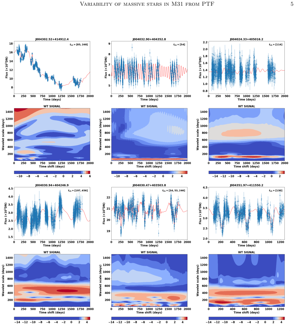
The load-bearing tool is a continuous wavelet transform with a Morlet wavelet applied to light curves that have been gap-filled by a Gaussian Process reconstruction using a critical filter, an approach imported from an earlier study of red supergiants. The wavelet transform maps correlation power as a function of both timescale and time, allowing a characteristic timescale $t_{\rm ch}$ to be extracted for signals that are periodic, stochastic, or transient. The reconstruction is limited to a maximum resolution of about 3 days, so reported long-baseline timescales are only trusted when $t_{\rm ch}$ exceeds 10 days. The transform normalization ($1/a$) makes the square root of the correlation power equal to the signal amplitude in flux units, which is then compared with empirically measured noise floors to reject timescales consistent with photometric noise. For short timescales, a 60-night block with resolution of about 30 minutes is analyzed separately.
What would settle it
Take a few of the 356 stars with measured $t_{\rm ch} \geq 10$ days and compare their reconstructed wavelet spectra against well-sampled continuous light curves from space-based photometry (for example, TESS sectors or K2 campaigns covering similar or longer baselines): if the independently measured periodograms or wavelet spectra lack the timescales claimed by the Gaussian Process reconstruction, the reported $t_{\rm ch}$ values would fail to represent the true variability.
Extended reading notes
Core claim
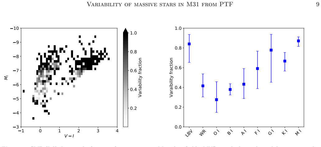
The central claim is that massive stars in M31 are almost universally variable, and that the pattern of their variability—its prevalence, amplitude, and characteristic timescale—is organized by spectral type in a way that current stellar models can broadly reproduce. From a spectroscopically typed sample of 491 stars, the paper finds that the observed variability fraction climbs from early spectral types to nearly 100% for M supergiants. The RMS amplitude is systematically larger for red evolved stars than for blue ones. The wavelet-derived characteristic timescale $t_{\rm ch}$ separates the population: cool supergiants sit at hundreds of days or more, while hotter stars cluster around tens of days but extend to both longer and shorter values. For luminous blue variables, the combination of short characteristic timescales and few-percent amplitudes is interpreted as stochastic microvariability driven by envelope convection, in line with recent three-dimensional hydrodynamical simulations.
Load-bearing premise
The entire timescale analysis rests on the assumption that the Gaussian Process reconstruction faithfully preserves real variability power on timescales above about 10 days, because if the reconstruction smooths away genuine short-timescale signal or introduces spurious correlated power, the reported characteristic timescales and their spectral-type trends would be artifacts.
Editorial extensions
If this is right
- Variability in M31's massive-star population is common and becomes nearly universal among cool supergiants, so any complete model of late-stage massive-star evolution must account for such pervasive photometric variation.
- The trend of larger amplitudes in red evolved stars on timescales of hundreds of days supports pulsation (likely fundamental and first-overtone modes) as a dominant driver in cool supergiants.
- The wavelet timescales of the hotter massive stars, often tens of days, are consistent with a mixture of opacity-driven pulsation, rotational modulation, and possibly stochastic low-frequency variability from internal gravity waves.
- The detection of 13 stars with 0.1–10 day variability at a few percent amplitude shows that ground-based surveys can find short-timescale variability in the brightest massive stars, providing a bridge to space-based studies with TESS.
Reading between the lines
- If the Gaussian Process reconstruction tends to smooth over low-amplitude, short-timescale fluctuations, the true frequency of short-timescale variables in M31 could be higher than the 13 stars reported here; a targeted TESS-like campaign on the brightest M31 supergiants could test this.
- The same wavelet-plus-Gaussian-Process pipeline could be applied to other Local Group galaxies with comparable time-domain coverage, allowing a first direct comparison of massive-star variability across metallicity environments.
- The two stars dropped for showing sub-resolution variability hint that the population of very short-timescale variables is partially hidden by the 3-day reconstruction limit; a higher-resolution reconstruction of those specific light curves could verify whether their true timescales fall in the 1–3 day range.
Signed reviews
Editorial analysis
A structured set of objections, weighed in public.
Referee Report
Summary. This paper presents a photometric variability study of 1050 spectroscopically classified massive stars in M31 using roughly five years of iPTF R-band forced photometry. After applying a magnitude cut and a noise-floor-based variability selection, the authors retain 491 variables, and through a Gaussian-process reconstruction of the unevenly sampled light curves plus a Morlet wavelet transform they derive characteristic variability timescales t_ch for 356 stars on timescales above 10 days. The three headline results are: (1) the detected variability fraction increases from early to late spectral types, approaching 100% for M supergiants; (2) redder stars (V-I > 1.5) show larger RMS amplitudes than bluer stars; and (3) cool supergiants have longer t_ch (typically hundreds of days) than hotter stars (typically tens of days), with an additional high-cadence analysis of a 60-night block yielding short timescales of 0.1-10 days for 13 stars.
Significance. If the t_ch map survives scrutiny, this is the first comprehensive characterization of massive-star variability in M31 across all spectral types, and the first wavelet-based characteristic-timescale map in the upper CMD of an external galaxy. The study extends Paper I's RSG analysis to the full massive-star population, provides a machine-readable catalog (Table 2) and publicly hosted light curves on DataLab, uses binomial confidence intervals on the variability fractions, gives a validation appendix for the wavelet extraction on simulated signals, and carries out visual inspection of all reconstructed light curves. The agreement with the M51 results of Conroy et al. (2018) on the variability-fraction and amplitude maps lends external support to those claims. The central t_ch claim, however, rests entirely on the fidelity of the Gaussian-process reconstruction on the real iPTF sampling; the validation gap described below is the main barrier to accepting the reported timescale trends at face value.
major comments (2)
- [§3.2, Appendix C] The Gaussian-Process reconstruction that underpins every t_ch measurement is validated in Appendix C only against simulated light curves with a uniform 2.5-day cadence, a gap-free baseline, high signal-to-noise, and signals that are exactly Morlet wavelets, whereas the actual iPTF data (Section 2.2) have irregular cadence and multi-month seasonal gaps over the five-year baseline. Because the critical filter infers both the signal and its power spectrum, the smoothness prior could bridge seasonal gaps with spurious long-timescale correlated power, and the two sources dropped in Section 3.2 (J004026.84+403504.6 and J004509.86+413031.5) show that genuine variability can be lost when it falls near the 3-day resolution. Since the cool-versus-hot t_ch trend in Figs. 9-10 is the paper's central novel claim, I ask that the recovery tests be redone on the actual iPTF time grid (or a representative gap-structured grid) with injected signals spanning the 10-1200 day range, including sines and red noise at the measured noise levels, and that the recovered t_ch be reported as a function of input timescale, spectral type, and signal-to-noise.
- [§3.2, Table 2, Figs. 9-11] The t_ch values in Table 2 and the distributions in Fig. 10 are reported without uncertainties, yet the method contains three sources of measurement error: the 5-sigma island-detection threshold, the automated island finder's fragmentation or merging of connected power regions, and the amplitude-versus-noise filter based on the Fig. 3 curve. The fragmentation is visible already in Table 2, where J003953.55+402827.7 is assigned 1130 and 1131 days as separate timescales. A modest change in the threshold, the wavelet scale grid, or the GP resolution could split or merge islands and move a star between the 'tens of days' and 'hundreds of days' regimes on which the spectral-type comparison in Fig. 10 rests; I ask for a robustness analysis (e.g., threshold variation or GP-posterior-based uncertainties) so that the trend claims carry a quantitative statement of precision.
minor comments (7)
- [Fig. 6, §4.2.3] The right-panel axis label in Fig. 6 reads 'Varaibility fraction' and should read 'Variability fraction'; the same misspelling ('varaibility') appears in Section 4.2.3 in 'Characterization of observed photometric varaibility in LBVs based on a large sample size'.
- [§3.2, Table 2] The machine-readable table should include the t_ch-specific amplitude (defined in Section 3.2 as alpha P^{1/2}) alongside each t_ch, since the text notes that some rows contain multiple t_ch values arising from fragmentation of a single connected island; this would allow readers to apply their own amplitude-versus-noise filter.
- [§3.2] The sentence stating that the two sources were 'vetted out' is ambiguous; 'dropped from the long-baseline t_ch analysis and re-examined in the high-cadence block' would be more precise, since Section 4.1 later includes them among the 13 short-timescale stars.
- [§3.3, Fig. 3] The high-cadence noise threshold is set to a constant 100 DN, while Fig. 3 shows that the noise estimates vary with timescale near the 60-day baseline; a short statement of the resulting systematic uncertainty in the short-t_ch detections for the 13 stars would strengthen the claim.
- [Appendix C] The calibration factor alpha = 1.7 x pixel/2.5 days should be explicitly identified as the conversion applied to the real light curves when computing t_ch-specific amplitudes in Section 3.2, as the text currently introduces it only as a scaling factor.
- [§4.2.1, Fig. 6] The variability-fraction map would be more informative with completeness-corrected fractions or at least the number of non-variable stars per spectral-type bin, since the early-type fractions are lower limits set by the Fig. 1 noise floor; the existing caveat in the text is helpful, but the figure itself does not convey this.
- [§3.1, Fig. 1] The functional form of the orange noise line, which defines the variability selection in Section 3.1 and is reused in Fig. 3, is not given in the text or in a table; quoting it would improve reproducibility.
Circularity Check
No significant circularity: the variability fractions, amplitudes, and tch maps are observational characterizations calibrated against external noise estimates and simulation tests, not predictions reduced to fitted inputs.
full rationale
The paper is an observational characterization of iPTF light curves rather than a derivation in which an output is constructed from its own input. Variability selection (Sect. 3.1) uses the Paper I noise floor ('The orange line shows the noise level of PTF from Paper I, which was computed considering only stars without PTF-detectable variability and with ⟨mR⟩ < 20 and extrapolated to fainter stars'), but this is a published, externally determined calibration curve, not a parameter fitted to the current sample's target claims; stars are then classified by whether their measured RMS exceeds that floor. The tch analysis (Sect. 3.2) reconstructs light curves with the critical filter, applies a Morlet wavelet transform, identifies islands above a 5σ background threshold, and filters against noise estimates from static stars; the amplitude calibration constant α is set using simulated wavelet signals in Appendix C, independent of the actual stellar light curves. The central claims (variability fraction increasing toward later types, redder stars having larger RMS amplitudes, cool supergiants having longer tch) are direct summaries of the resulting measurements and are benchmarked against independent work (Conroy et al. 2018, Dorn-Wallenstein et al. 2019) and external theoretical predictions. The only self-citations are to Paper I for the noise curve and for having previously implemented the reconstruction; these do not encode the present results. The statement that LBVs have a variability fraction near 100% is explicitly definitional ('LBVs by definition are variables') but is not load-bearing for the paper's main conclusions. Potential limitations of the Gaussian-process reconstruction for uneven sampling are correctness and robustness concerns, not circularity, because no target quantity was fitted and then re-predicted.
Assumptions & free parameters
free parameters (4)
- Wavelet amplitude calibration factor =
1.7 x (pixel size / 2.5 days)
- Wavelet power threshold =
5 sigma above background (background = mean of pixels below 75th percentile)
- High-cadence noise threshold =
100 DN (constant)
- GP reconstruction resolution =
~3 days (long baseline), ~30 minutes (high-cadence block)
assumptions (6)
- domain assumption The adopted distance modulus to M31 is 24.36 mag (Vilardell et al. 2010).
- domain assumption The foreground reddening toward M31 is E(B-V) = 0.062 mag (Schlegel et al. 1998), with no correction for internal M31 extinction.
- domain assumption Spectral types and M31 membership flags from Massey et al. (2016, MNS16) are correct.
- domain assumption The forced photometry on iPTF difference images, calibrated via template-image PSF photometry with a 2-inch search radius, yields accurate R-band fluxes for the sample stars.
- domain assumption The photometric noise model (orange line in Fig. 1) from Paper I, computed from stars deemed non-variable in that earlier study, is applicable to the M31 sample and its extrapolation to fainter magnitudes is valid.
- domain assumption The Gaussian Process reconstruction with the critical filter (Oppermann et al. 2013) preserves the true variability power at timescales above 10 days, neither smoothing away real signal nor creating spurious power.
Cite this review
Pith. "Pith review of Variability of massive stars in M31 from the Palomar Transient Factory." pith.science (2026). https://pith.science/paper/SMDDOBGM
@misc{pith2026190802439,
  author       = {Pith},
  title        = {Pith review of: Variability of massive stars in M31 from the Palomar Transient Factory},
  year         = {2026},
  howpublished = {\url{https://pith.science/paper/SMDDOBGM}},
  note         = {Machine review of arXiv:1908.02439}
}
read the original abstract
Using data from the (intermediate) Palomar Transient Factory (iPTF), we characterize the time variability of ~500 massive stars in M31. Our sample is those stars which are spectrally typed by Massey and collaborators, including Luminous Blue Variables, Wolf-Rayets, and warm and cool supergiants. We use the high-cadence, long-baseline (~5 years) data from the iPTF survey, coupled with data-processing tools that model complex features in the light curves. We find widespread photometric (R-band) variability in the upper Hertzsprung Russell diagram (or CMD) with an increasing prevalence of variability with later spectral types. Red stars (V-I>1.5) exhibit larger amplitude fluctuations than their bluer counterparts. We extract a characteristic variability timescale, tch, via wavelet transformations that are sensitive to both continuous and localized fluctuations. Cool supergiants are characterized by longer timescales (>100 days) than the hotter stars. The latter have typical timescales of tens of days but cover a wider range, from our resolution limit of a few days to longer than 100 days timescales. Using a 60-night block of data straddling two nights with a cadence of around 2 minutes, we extracted tch in the range 0.1--10 days with amplitudes of a few percent for 13 stars. Though there is broad agreement between the observed variability characteristics in the different parts of the upper CMD with theoretical predictions, detailed comparison requires models with a more comprehensive treatment of the various physical processes operating in these stars such as pulsation, subsurface convection, and the effect of binary companions.
Figures


Figures from the paper (21 more)




Reference graph
Works this paper leans on
-
[1]
, " * write output.state after.block = add.period write newline
ENTRY address archivePrefix author booktitle chapter doi edition editor eprint howpublished institution journal key month note number organization pages publisher school series title misctitle type volume year version url label extra.label sort.label short.list INTEGERS output.state before.all mid.sentence after.sentence after.block FUNCTION init.state.co...
-
[2]
write newline
" write newline "" before.all 'output.state := FUNCTION format.doi doi empty "" "doi:" doi * if FUNCTION format.url url empty "" new.block "" url * "" * if FUNCTION format.eprint eprint empty "" archivePrefix empty "" archivePrefix ":" * if eprint field.or.null * if FUNCTION format.pid eprint empty format.doi format.eprint if FUNCTION n.dashify 't := "" t...
-
[3]
thebibliography [1] 20pt to REFERENCES 6pt =0pt 10pt plus 3pt =0pt =0pt =1pt plus 1pt =0pt =0pt -12pt =13pt plus 1pt =20pt =13pt plus 1pt \@M =10000 =-1.0em =0pt =0pt 0pt =0pt =1.0em @enumiv\@empty 10000 10000 `\.\@m \@noitemerr \@latex@warning Empty `thebibliography' environment \@ifnextchar \@reference \@latexerr Missing key on reference command Each re...
-
[4]
Abbott , D. C. 1982, , 263, 723
1982
-
[5]
2011, New Astronomy, 16, 421
Abolmasov , P. 2011, New Astronomy, 16, 421
2011
-
[6]
Aerts , C., & Rogers , T. M. 2015, , 806, L33
2015
-
[7]
M., S \' mon-D \' az , S., et al
Aerts , C., Bowman , D. M., S \' mon-D \' az , S., et al. 2018, , 476, 1234
2018
-
[8]
P., Tollerud , E
Astropy Collaboration , Robitaille , T. P., Tollerud , E. J., et al. 2013, , 558, A33
2013
Show all 125 references
-
[9]
Bailer-Jones , C. A. L., Rybizki , J., Fouesneau , M., Mantelet , G., & Andrae , R. 2018, , 156, 58
2018
-
[10]
C., Kulkarni , S
Bellm , E. C., Kulkarni , S. R., Graham , M. J., et al. 2019, , 131, 018002
2019
-
[11]
D., Harper , G
Bennett , P. D., Harper , G. M., Brown , A., & Hummel , C. A. 1996, , 471, 454
1996
-
[12]
C., Stanek , K
Bird , J. C., Stanek , K. Z., & Prieto , J. L. 2009, , 695, 874
2009
-
[13]
1999 a , , 512, 711
Bono , G., Caputo , F., Castellani , V., & Marconi , M. 1999 a , , 512, 711
1999
-
[14]
Bono , G., Marconi , M., & Stellingwerf , R. F. 1999 b , , 122, 167
1999
-
[15]
M., Burssens , S., Pedersen , M
Bowman , D. M., Burssens , S., Pedersen , M. G., et al. 2019, Nature Astronomy, 320
2019
-
[16]
1978, , 65, 363
Burki , G., Maeder , A., & Rufener , F. 1978, , 65, 363
1978
-
[17]
2019, arXiv e-prints, arXiv:1904.02161
Cantiello , M., & Braithwaite , J. 2019, arXiv e-prints, arXiv:1904.02161
2019 arXiv
-
[18]
2009, , 499, 279
Cantiello , M., Langer , N., Brott , I., et al. 2009, , 499, 279
2009
-
[19]
2018, , 859, 140
Chen , X., Deng , L., de Grijs , R., Wang , S., & Feng , Y. 2018, , 859, 140
2018
-
[20]
2009, , 506, 1351
Chiavassa , A., Plez , B., Josselin , E., & Freytag , B. 2009, , 506, 1351
2009
-
[21]
U., & Kim , J
Chun , S.-H., Yoon , S.-C., Jung , M.-K., Kim , D. U., & Kim , J. 2018, , 853, 79
2018
-
[22]
2018, , 864, 111
Conroy , C., Strader , J., van Dokkum , P., et al. 2018, , 864, 111
2018
-
[23]
A., Cox , N
Cordiner , M. A., Cox , N. L. J., Evans , C. J., et al. 2011, , 726, 39
2011
-
[24]
N., Morgan , S
Cox , A. N., Morgan , S. M., Rogers , F. J., & Iglesias , C. A. 1992, , 393, 272
1992
-
[25]
2005, Journal of Parallel and Distributed Computing, 65, 1108
Dalc\'in, L., Paz, R., & Storti, M. 2005, Journal of Parallel and Distributed Computing, 65, 1108 . http://www.sciencedirect.com/science/article/pii/S0743731505000560
2005
-
[26]
Z., Levesque , E
Dorn-Wallenstein , T. Z., Levesque , E. M., & Davenport , J. R. A. 2019, arXiv e-prints, arXiv:1901.09930
2019 arXiv
-
[27]
R., Dufton , P
Dunstall , P. R., Dufton , P. L., Sana , H., et al. 2015, , 580, A93
2015
-
[28]
A., Moskalik , P., & Pamyatnykh , A
Dziembowski , W. A., Moskalik , P., & Pamyatnykh , A. A. 1993, , 265, 588
1993
-
[29]
1996, , 112, 1709
Foster , G. 1996, , 112, 1709
1996
-
[30]
Freyer , T., Hensler , G., & Yorke , H. W. 2003, , 594, 888
2003
-
[31]
2006, , 638, 262
---. 2006, , 638, 262
2006
-
[32]
L., Galyagin , D., Sokoloff , D., & Soon , W
Frick , P., Baliunas , S. L., Galyagin , D., Sokoloff , D., & Soon , W. 1997, , 483, 426
1997
-
[33]
Gaia Collaboration , Prusti , T., de Bruijne , J. H. J., et al. 2016, , 595, A1
2016
-
[34]
2018 a , arXiv e-prints, arXiv:1804.09382
Gaia Collaboration , Eyer , L., Rimoldini , L., et al. 2018 a , arXiv e-prints, arXiv:1804.09382
2018 arXiv
-
[35]
Gaia Collaboration , Brown , A. G. A., Vallenari , A., et al. 2018 b , , 616, A1
2018
-
[36]
2018 c , , 616, A1
---. 2018 c , , 616, A1
2018
-
[37]
2010, , 463, 203
Governato , F., Brook , C., Mayer , L., et al. 2010, , 463, 203
2010
-
[38]
H., & Li , Y
Guo , J. H., & Li , Y. 2002, , 565, 559
2002
-
[39]
M., Dettmar , R.-J., Beckman , J
Haffner , L. M., Dettmar , R.-J., Beckman , J. E., et al. 2009, Reviews of Modern Physics, 81, 969
2009
-
[40]
1997, , 327, 224
Heger , A., Jeannin , L., Langer , N., & Baraffe , I. 1997, , 327, 224
1997
-
[41]
1953, , 118, 353
Hubble , E., & Sandage , A. 1953, , 118, 353
1953
-
[42]
M., & Davidson , K
Humphreys , R. M., & Davidson , K. 1994, , 106, 1025
1994
-
[43]
M., Davidson , K., Hahn , D., Martin , J
Humphreys , R. M., Davidson , K., Hahn , D., Martin , J. C., & Weis , K. 2017, , 844, 40
2017
-
[44]
Hunter, J. D. 2007, Computing In Science & Engineering, 9, 90
2007
-
[45]
2015, , 813, 74
Jiang , Y.-F., Cantiello , M., Bildsten , L., Quataert , E., & Blaes , O. 2015, , 813, 74
2015
-
[46]
2018, , 561, 498
Jiang , Y.-F., Cantiello , M., Bildsten , L., et al. 2018, , 561, 498
2018
-
[47]
2001--, SciPy : Open source scientific tools for Python , , , http://www.scipy.org/
Jones, E., Oliphant, T., Peterson, P., et al. 2001--, SciPy : Open source scientific tools for Python , , , http://www.scipy.org/. http://www.scipy.org/
2001
-
[48]
2010, Society of Photo-Optical Instrumentation Engineers (SPIE) Conference Series, Vol
Kaiser , N., Burgett , W., Chambers , K., et al. 2010, Society of Photo-Optical Instrumentation Engineers (SPIE) Conference Series, Vol. 7733, The Pan-STARRS wide-field optical/NIR imaging survey , 77330E
2010
-
[49]
Kervella , P., Decin , L., Richards , A. M. S., et al. 2018, , 609, A67
2018
-
[50]
J., & Glatzel , W
Kiriakidis , M., Fricke , K. J., & Glatzel , W. 1993, , 264, 50
1993
-
[51]
L., Szab \'o , G
Kiss , L. L., Szab \'o , G. M., & Bedding , T. R. 2006, , 372, 1721
2006
-
[52]
Z., Soszy \'n ski , I., et al
Kourniotis , M., Bonanos , A. Z., Soszy \'n ski , I., et al. 2014, , 562, A125
2014
-
[53]
R., Surace , J., Grillmair , C
Laher , R. R., Surace , J., Grillmair , C. J., et al. 2014, , 126, 674
2014
-
[54]
Lamers , H. J. G. L. M., Bastiaanse , M. V., Aerts , C., & Spoon , H. W. W. 1998, , 335, 605
1998
-
[55]
M., Kulkarni , S
Law , N. M., Kulkarni , S. R., Dekany , R. G., et al. 2009, , 121, 1395
2009
-
[56]
H., Riffeser , A., Koppenhoefer , J., et al
Lee , C. H., Riffeser , A., Koppenhoefer , J., et al. 2012, , 143, 89
2012
-
[57]
Levesque , E. M. 2017, Astrophysics of Red Supergiants , doi:10.1088/978-0-7503-1329-2
2017 doi
-
[58]
Li , Y., & Gong , Z. G. 1994, , 289, 449
1994
-
[59]
Lilly , J. M. 2017, arXiv e-prints, arXiv:1703.04882
2017 arXiv
-
[60]
1984, , 133, 307
Lovy , D., Maeder , A., Noels , A., & Gabriel , M. 1984, , 133, 307
1984
-
[61]
1980, , 90, 311
Maeder , A. 1980, , 90, 311
1980
-
[62]
1985, , 147, 300
---. 1985, , 147, 300
1985
-
[63]
J., Laher , R
Masci , F. J., Laher , R. R., Rebbapragada , U. D., et al. 2017, , 129, 014002
2017
-
[64]
2003, , 41, 15
Massey , P. 2003, , 41, 15
2003
-
[65]
2013, New Astronomy Reviews, 57, 14
---. 2013, New Astronomy Reviews, 57, 14
2013
-
[66]
Massey , P., & Evans , K. A. 2016, , 826, 224
2016
-
[67]
T., Olsen , K
Massey , P., McNeill , R. T., Olsen , K. A. G., et al. 2007, , 134, 2474
2007
-
[68]
F., & Levesque , E
Massey , P., Neugent , K. F., & Levesque , E. M. 2017, Philosophical Transactions of the Royal Society of London Series A, 375, 20160267
2017
-
[69]
F., & Smart , B
Massey , P., Neugent , K. F., & Smart , B. M. 2016, , 152, 62
2016
-
[70]
Massey , P., Olsen , K. A. G., Hodge , P. W., et al. 2006, , 131, 2478
2006
-
[71]
Matzner , C. D. 2002, , 566, 302
2002
-
[72]
2010, in Proceedings of the 9th Python in Science Conference, ed
McKinney, W. 2010, in Proceedings of the 9th Python in Science Conference, ed. S. van der Walt & J. Millman, 51 -- 56
2010
-
[73]
H., et al
Mehner , A., Baade , D., Groh , J. H., et al. 2017, , 608, A124
2017
-
[74]
Moffat , A. F. J., & Robert , C. 1991, in IAU Symposium, Vol. 143, Wolf-Rayet Stars and Interrelations with Other Massive Stars in Galaxies, ed. K. A. van der Hucht & B. Hidayat , 109
1991
-
[75]
R., & Lester , J
Neilson , H. R., & Lester , J. B. 2008, , 684, 569
2008
-
[76]
2019, Galaxies, 7, 74
Neugent , K., & Massey , P. 2019, Galaxies, 7, 74
2019
-
[77]
F., & Massey , P
Neugent , K. F., & Massey , P. 2014, , 789, 10
2014
-
[78]
F., Massey , P., & Georgy , C
Neugent , K. F., Massey , P., & Georgy , C. 2012, , 759, 11
2012
-
[79]
2013, , 51, 457
Nomoto , K., Kobayashi , C., & Tominaga , N. 2013, , 51, 457
2013
-
[80]
R., & En lin , T
Oppermann , N., Selig , M., Bell , M. R., & En lin , T. A. 2013, , 87, 032136
2013
-
[81]
2019, arXiv e-prints, arXiv:1904.07878
Ouchi , R., & Maeda , K. 2019, arXiv e-prints, arXiv:1904.07878
2019 arXiv
-
[82]
R., Lennon , D
Patrick , L. R., Lennon , D. J., Britavskiy , N., et al. 2019, , 624, A129
2019
-
[83]
2013, , 208, 4
Paxton , B., Cantiello , M., Arras , P., et al. 2013, , 208, 4
2013
-
[84]
2015, , 220, 15
Paxton , B., Marchant , P., Schwab , J., et al. 2015, , 220, 15
2015
-
[85]
G., Chowdhury , S., Johnston , C., et al
Pedersen , M. G., Chowdhury , S., Johnston , C., et al. 2019, , 872, L9
2019
-
[86]
H., Friend , D
Poe , C. H., Friend , D. B., & Cassinelli , J. P. 1989, , 337, 888
1989
-
[87]
2002, , 52, 397
Pojmanski , G. 2002, , 52, 397
2002
-
[88]
L., Stanek , K
Prieto , J. L., Stanek , K. Z., Kochanek , C. S., et al. 2008, , 673, L59
2008
-
[89]
R., Law , N
Rau , A., Kulkarni , S. R., Law , N. M., et al. 2009, , 121, 1334
2009
-
[90]
2019, , 241, 35
Ren , Y., Jiang , B.-W., Yang , M., & Gao , J. 2019, , 241, 35
2019
-
[91]
E., Ellis , R
Robertson , B. E., Ellis , R. S., Furlanetto , S. R., & Dunlop , J. S. 2015, , 802, L19
2015
-
[92]
1976, , 26, 275
Rufener , F. 1976, , 26, 275
1976
-
[93]
1978, , 31, 179
Rufener , F., Maeder , A., & Burki , G. 1978, , 31, 179
1978
-
[94]
E., de Koter , A., et al
Sana , H., de Mink , S. E., de Koter , A., et al. 2012, Science, 337, 444
2012
-
[95]
E., Garrison , R
Schild , R. E., Garrison , R. F., & Hiltner , W. A. 1983, , 88, 67
1983
-
[96]
J., Finkbeiner , D
Schlegel , D. J., Finkbeiner , D. P., & Davis , M. 1998, , 500, 525
1998
-
[97]
R., Junklewitz , H., et al
Selig , M., Bell , M. R., Junklewitz , H., et al. 2013, , 554, A26
2013
-
[98]
A., et al
Sim \'o n-D \' az , S., Aerts , C., Urbaneja , M. A., et al. 2018, , 612, A40
2018
-
[99]
D., Gilfanov , M., Kupfer , T., et al
Soraisam , M. D., Gilfanov , M., Kupfer , T., et al. 2017, , 599, A48
2017
-
[100]
D., Bildsten , L., Drout , M
Soraisam , M. D., Bildsten , L., Drout , M. R., et al. 2018, , 859, 73
2018
-
[101]
2014, , 570, A3
Sperauskas , J., Za c s , L., Raudeli \= u nas , S., Musaev , F., & Puzin , V. 2014, , 570, A3
2014
-
[102]
T., Bonanos , A
Spetsieri , Z. T., Bonanos , A. Z., Kourniotis , M., et al. 2018, , 618, A185
2018
-
[103]
Stetson , P. B. 1987, , 99, 191
1987
-
[104]
1990, , 102, 932
---. 1990, , 102, 932
1990
-
[105]
1969, , 156, 541
Stothers , R. 1969, , 156, 541
1969
-
[106]
Stothers , R., & Leung , K. C. 1971, , 10, 290
1971
-
[107]
Stothers , R. B. 2010, , 725, 1170
2010
-
[108]
B., & Chin , C.-W
Stothers , R. B., & Chin , C.-W. 1995, , 451, L61
1995
-
[109]
M., Stanek , K
Szczygie , D. M., Stanek , K. Z., Bonanos , A. Z., et al. 2010, , 140, 14
2010
-
[110]
Townsend , R. H. D., & Teitler , S. A. 2013, , 435, 3406
2013
-
[111]
2003, , 53, 291
Udalski , A. 2003, , 53, 291
2003
-
[112]
C., & Varoquaux, G
van der Walt, S., Colbert, S. C., & Varoquaux, G. 2011, Computing In Science & Engineering, 13, 22
2011
-
[113]
van Genderen , A. M. 2001, , 366, 508
2001
-
[114]
M., de Groot , M., & Sterken , C
van Genderen , A. M., de Groot , M., & Sterken , C. 1997, , 124, 517
1997
-
[115]
M., Sterken , C., & Jones , A
van Genderen , A. M., Sterken , C., & Jones , A. F. 2004, , 419, 667
2004
-
[116]
M., & The , P
van Genderen , A. M., & The , P. S. 1984, , 39, 317
1984
-
[117]
M., Veijgen , S
van Genderen , A. M., Veijgen , S. R. G., & van der Hucht , K. A. 2013, , 345, 133
2013
-
[118]
2005, , 43, 769
Veilleux , S., Cecil , G., & Bland-Hawthorn , J. 2005, , 43, 769
2005
-
[119]
L., & Guinan , E
Vilardell , F., Ribas , I., Jordi , C., Fitzpatrick , E. L., & Guinan , E. F. 2010, , 509, A70
2010
-
[120]
Vreux , J. M. 1985, , 97, 274
1985
-
[121]
G., McKee , C
Wolfire , M. G., McKee , C. F., Hollenbach , D., & Tielens , A. G. G. M. 2003, , 587, 278
2003
-
[122]
Wright , K. O. 1977, , 71, 152
1977
-
[123]
Yang , M., & Jiang , B. W. 2011, , 727, 53
2011
-
[124]
2012, , 754, 35
---. 2012, , 754, 35
2012
-
[125]
2010, , 717, L62
Yoon , S.-C., & Cantiello , M. 2010, , 717, L62
2010
Reviewed August 14, 2026 · model on record in the stance chip above.
Discussion (0). Continue with ORCID to comment.