Adaptation of the hybrid fictitious domain-immersed boundary method for Reynolds-averaged turbulence modeling
Pith reviewed 2026-06-27 23:07 UTC · model grok-4.3
The pith
A hybrid fictitious domain-immersed boundary method adapted for RANS turbulence models produces results consistent with body-fitted CFD across Reynolds numbers from 10 to 10^6.
A machine-rendered reading of the paper's core claim, the machinery that carries it, and where it could break.
Core claim
The hybrid fictitious domain-immersed boundary forcing terms and wall-function treatment can be combined with the steady SIMPLE algorithm to produce an IB-aware RANS solver whose outputs remain consistent with body-fitted CFD for two-equation models, Reynolds numbers spanning five orders of magnitude, and both canonical and general geometries.
What carries the argument
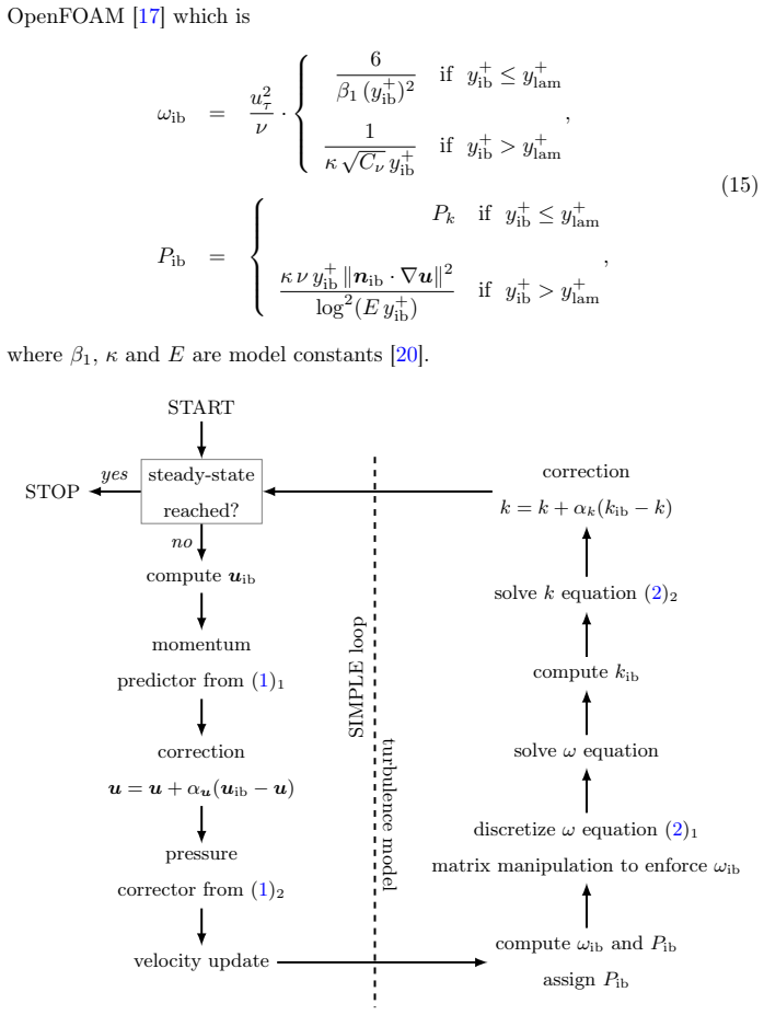
Hybrid fictitious domain-immersed boundary forcing terms with wall-function treatment inside the steady SIMPLE algorithm for RANS equations.
If this is right
- CFD-based topology optimization can proceed without remeshing at each design iteration.
- The method applies directly to the standard two-equation RANS closures over the full practical Reynolds-number range.
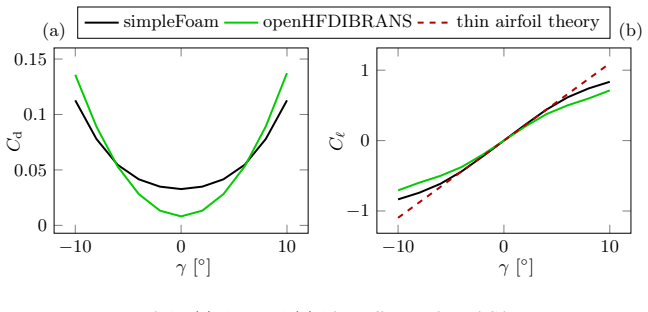
- Results remain consistent on both simple benchmarks and more general shapes such as airfoils at varying incidence.
- The implementation is open-source and already integrated with an existing CFD library.
Where Pith is reading between the lines
- The same forcing structure could be tested on unsteady or higher-fidelity turbulence closures.
- Computational savings would be largest in optimization loops that require dozens or hundreds of flow evaluations.
- Accuracy on very thin or highly curved immersed surfaces remains an open practical question.
Load-bearing premise
The immersed-boundary forcing and wall-function treatment stay stable and accurate for arbitrary immersed geometries when the flow is solved with the steady SIMPLE algorithm.
What would settle it
A benchmark case with an arbitrary immersed shape at Reynolds number 10^6 where the immersed-boundary RANS solution deviates measurably from an equivalent body-fitted solution in skin friction or separation location.
Figures


read the original abstract
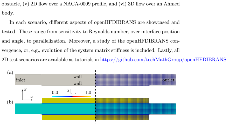
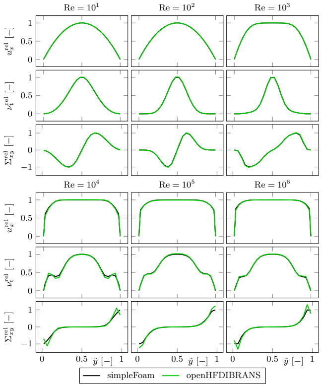
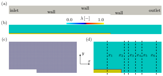
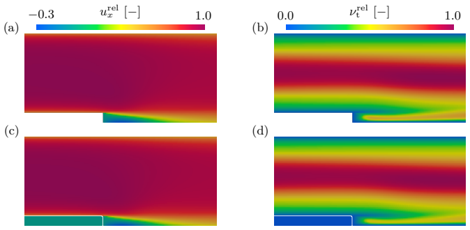
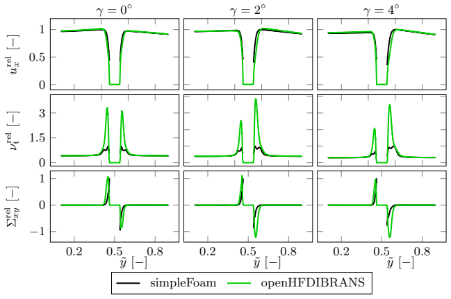
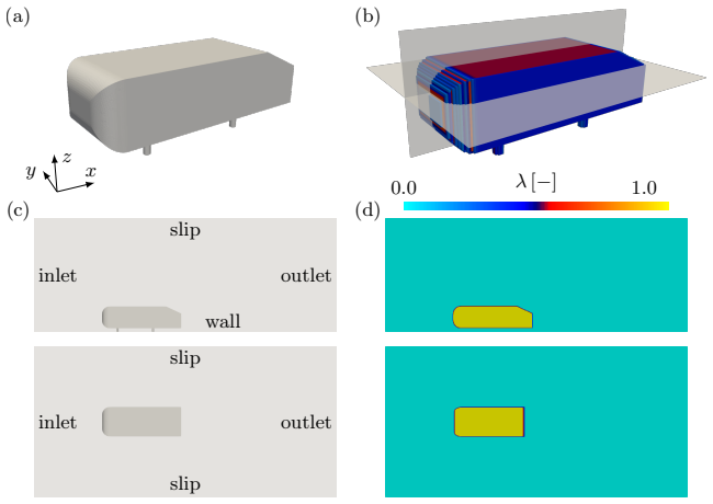
Engineering practice often calls for shape or topology optimization (TO) of fluid defining components, while the ever-increasing computing power allows the optimized cost functions to be based on computational fluid dynamics (CFD). However, a common bottleneck in CFD-based TO frameworks is the requirement for frequent remeshing. In order to alleviate this bottleneck, we propose an adaptation of an immersed boundary (IB) method variant, the hybrid fictitious domain-immersed boundary method, to leverage Reynolds-averaged Navier-Stokes (RANS) equations and wall function. The main contribution of the present work lies in the design and open-source implementation of the IB-aware steady-state solution of the RANS equations via the SIMPLE algorithm in the OpenFOAM library. For the most common two-equation RANS models, Reynolds numbers from $10^1$ to $10^6$, and several benchmarks, such as flow over a backwards facing step or an Ahmed body, the framework gives results consistent with the standard body-fitted CFD. Furthermore, given the intended application in TO, special emphasis is placed on the robustness and applicability of the approach to general geometries, which is tested on a NACA profile under various angles of attack.
Editorial analysis
A structured set of objections, weighed in public.
Referee Report
Summary. The manuscript adapts the hybrid fictitious domain-immersed boundary (IB) method to Reynolds-averaged Navier-Stokes (RANS) turbulence modeling with wall functions. The central contribution is an open-source implementation of an IB-aware steady-state RANS solver using the SIMPLE algorithm within OpenFOAM. The authors claim that, for standard two-equation RANS models and Reynolds numbers from 10^1 to 10^6, the approach produces results consistent with body-fitted CFD on benchmarks including the backwards-facing step, Ahmed body, and NACA airfoil at varying angles of attack, with emphasis on robustness for general geometries to enable topology optimization without remeshing.
Significance. If the consistency and robustness claims hold with quantitative support, the work removes a key practical obstacle (repeated remeshing) in CFD-driven shape and topology optimization of fluid components. The OpenFOAM implementation and focus on steady SIMPLE coupling for RANS are practical strengths that could facilitate adoption in engineering workflows.
major comments (2)
- [Abstract] Abstract: the headline claim that 'the framework gives results consistent with the standard body-fitted CFD' for the listed benchmarks and Re range is load-bearing, yet no quantitative error metrics, coefficient comparisons, grid-convergence indices, or residual histories are supplied to allow verification of that consistency.
- [Abstract] Abstract (robustness paragraph): the extension to 'general geometries' required for topology optimization rests on the unshown stability and accuracy of the hybrid fictitious-domain IB forcing terms plus wall-function treatment when the immersed surface is non-smooth or multiply connected and the pressure-velocity coupling uses the steady SIMPLE algorithm; only the smooth NACA profile is mentioned as a test case.
minor comments (1)
- [Abstract] Abstract: the notation '$10^1$ to $10^6$' for Reynolds number could be clarified to indicate whether transitional regimes (where RANS applicability is limited) are included.
Simulated Author's Rebuttal
We thank the referee for the constructive feedback on our manuscript. We address each major comment below and have made revisions to strengthen the presentation of our results and claims.
read point-by-point responses
-
Referee: [Abstract] Abstract: the headline claim that 'the framework gives results consistent with the standard body-fitted CFD' for the listed benchmarks and Re range is load-bearing, yet no quantitative error metrics, coefficient comparisons, grid-convergence indices, or residual histories are supplied to allow verification of that consistency.
Authors: We agree that the abstract claim would be strengthened by quantitative support. The full manuscript presents visual comparisons and qualitative agreement in the results section for the backwards-facing step, Ahmed body, and NACA airfoil cases across the stated Re range. To address the concern directly, we will revise the abstract to include specific quantitative indicators such as relative errors in drag/lift coefficients and key flow quantities (e.g., reattachment length) where they are reported in the body of the paper. revision: yes
-
Referee: [Abstract] Abstract (robustness paragraph): the extension to 'general geometries' required for topology optimization rests on the unshown stability and accuracy of the hybrid fictitious-domain IB forcing terms plus wall-function treatment when the immersed surface is non-smooth or multiply connected and the pressure-velocity coupling uses the steady SIMPLE algorithm; only the smooth NACA profile is mentioned as a test case.
Authors: The robustness paragraph highlights the NACA profile at varying angles of attack because it directly tests the method under changing flow conditions relevant to optimization. However, the backwards-facing step and Ahmed body benchmarks explicitly include sharp edges, corners, and non-smooth surfaces, which exercise the IB forcing and wall-function treatment on non-smooth geometries under the steady SIMPLE algorithm. We will revise the abstract to explicitly reference these cases as supporting evidence for applicability to general (including non-smooth) geometries. revision: yes
Circularity Check
No circularity: implementation paper validated on external benchmarks
full rationale
The paper describes an adaptation of the hybrid fictitious domain-immersed boundary method to RANS equations with wall functions, implemented via the steady SIMPLE algorithm in OpenFOAM. Its central claim is empirical consistency with body-fitted CFD results across listed benchmarks (backwards-facing step, Ahmed body, NACA profile) for common two-equation models and Re 10^1–10^6. No derivation chain is present; the work consists of code-level modifications and direct numerical comparisons against independent external solvers. No equations reduce to fitted inputs by construction, no uniqueness theorems are imported via self-citation, and no ansatz or renaming is smuggled in. The extension to general geometries is asserted via the NACA tests but remains an empirical claim, not a self-referential derivation.
Axiom & Free-Parameter Ledger
axioms (1)
- domain assumption Standard two-equation RANS closures and wall functions remain valid when the near-wall treatment is replaced by immersed-boundary forcing.
Reference graph
Works this paper leans on
-
[1]
C. S. Peskin, Flow patterns around heart valves: A numerical method, Journal of Computational Physics 10 (1972) 252–271
1972
-
[2]
Mittal, J
R. Mittal, J. H. Seo, Origin and evolution of immersed boundary methods in computational fluid dynamics, Physical Review Fluids 8 (2023) 100501. 38
2023
-
[3]
Verzicco, Immersed boundary methods: Historical perspective and fu- ture outlook, Annual Review of Fluid Mechanics 55 (2023) 129–155
R. Verzicco, Immersed boundary methods: Historical perspective and fu- ture outlook, Annual Review of Fluid Mechanics 55 (2023) 129–155
2023
-
[4]
Kalitzin, G
G. Kalitzin, G. Iaccarino, Turbulence modeling in an immersed-boundary RANS method, Center for Turbulence Research Annual Research Briefs (2002) 415–426
2002
-
[5]
Capizzano, Turbulent wall model for immersed boundary methods, AIAA Journal 49 (2011) 2367–2381
F. Capizzano, Turbulent wall model for immersed boundary methods, AIAA Journal 49 (2011) 2367–2381
2011
-
[6]
Constant, S
B. Constant, S. Péron, H. Beaugendre, An improved immersed bound- ary method for turbulent flow simulations on cartesian grids, Journal of Computational Physics 435 (2021) 110240
2021
-
[7]
S.-G. Cai, J. Degrigny, J.-F. Boussuge, P. Sagaut, Coupling of turbulence wall models and immersed boundaries on cartesian grids, Journal of Com- putational Physics 429 (2021) 109995
2021
-
[8]
Constant, S
B. Constant, S. Péron, H. Beaugendre, C. Benoit, An improved immersed boundary method for turbulent flow simulations on cartesian grids: exten- sion of a global geometric approach for thin boundary layers and strong flow incidence, Journal of Computational Physics 519 (2024) 113441
2024
-
[9]
N.Troldborg, N.N.Sørensen, F.Zahle, Immersedboundarymethodfor the incompressible Reynolds Averaged Navier–Stokes equations, Computers and Fluids 237 (2022) 105340
2022
-
[10]
Fadlun, R
E. Fadlun, R. Verzicco, P. Orlandi, J. Mohd-Yusof, Combined immersed- boundary finite-difference methods for three-dimensional complex flow sim- ulations, Journal of Computational Physics 161 (2000) 35–60
2000
-
[11]
J. Kim, D. Kim, H. Choi, An immersed-boundary finite-volume method for simulations of flow in complex geometries, Journal of Computational Physics 171 (2001) 132–150. 39
2001
-
[12]
Uhlmann, An immersed boundary method with direct forcing for the simulation of particulate flows, Journal of Computational Physics 209 (2005) 448–476
M. Uhlmann, An immersed boundary method with direct forcing for the simulation of particulate flows, Journal of Computational Physics 209 (2005) 448–476
2005
-
[13]
Municchi, S
F. Municchi, S. Radl, Consistent closures for euler-lagrange models of bi-disperse gas-particle suspensions derived from particle-resolved direct numerical simulations, International Journal of Heat and Mass Transfer 111 (2017) 171–190
2017
-
[14]
M. Isoz, M. K. Šourek, O. Studeník, P. Kočí, Hybrid fictitious domain- immersed boundary solver coupled with discrete element method for simu- lations of flows laden with arbitrarily-shaped particles, Computers & Fluids 244 (2022) 105538
2022
-
[15]
Studeník, M
O. Studeník, M. Isoz, M. K. Šourek, P. Kočí, OpenHFDIB-DEM: An extension to OpenFOAM for CFD-DEM simulations with arbitrary particle shapes, SoftwareX 27 (2024) 101871
2024
-
[16]
M. K. Šourek, O. Studeník, M. Isoz, P. Kočí, A. P. York, Viscosity predic- tion for dense suspensions of non-spherical particles based on CFD-DEM simulations, Powder Technology 444 (2024) 120067
2024
-
[17]
Weller, C
H. Weller, C. Greenshields, W. B. et al., OpenFOAM, 2022. URL:https: //openfoam.org/
2022
-
[18]
Launder, D
B. Launder, D. Spalding, The numerical computation of turbulent flows, Computer Methods in Applied Mechanics and Engineering 3 (1974) 269– 289
1974
-
[19]
S. E. Tahry,k-ϵequation for compressible reciprocating engine flows, En- ergy 7 (1983) 345–353
1983
-
[20]
Wilcox, Turbulence modeling for CFD, 3 ed., DCW Industries, USA, 2006
D. Wilcox, Turbulence modeling for CFD, 3 ed., DCW Industries, USA, 2006. 40
2006
-
[21]
F. R. Menter, Improved two equationk-ωturbulence models for aerody- namic flows, Technical Report N93-22809, NASA, 1992
1992
-
[22]
T. H. Shih, W. Liou, A. Shabbir, Z. Yang, J. Zhu, A newk-ϵeddy viscosity model for high Reynolds number turbulent flows, Computer & Fluids 24 (1995) 227–238
1995
-
[23]
J.Bredberg, Onthewallboundaryconditionforturbulencemodels, Techni- cal Report Internal report 00/4, Chalmers University of Technology, Gote- borg, 2000
2000
-
[24]
Kubíčková, M
L. Kubíčková, M. Isoz, On reynolds-averaged turbulence modeling with im- mersed boundary method, in: D. Šimurda, T. Bodnár (Eds.), Proceedings of Topical Problems of Fluid Mechanics 2023, IT CAS, 2023, pp. 104–111
2023
-
[25]
Kalitzin, G
G. Kalitzin, G. Medic, G. Iaccarino, P. Durbin, Near-wall behavior of rans turbulence models and implications for wall functions, Journal of Computational Physics 204 (2005) 265–291
2005
-
[26]
Patankar, D
S. Patankar, D. Spalding, A calculation procedure for heat, mass and momentum transfer in three-dimensional parabolic flows, International Journal of Heat and Mass Transfer 15 (1972) 1787–1806
1972
-
[27]
Moukalled, M
F. Moukalled, M. Darwish, L. Mangani, The finite volume method in com- putational fluid dynamics: an advanced introduction with OpenFOAM and Matlab, 1 ed., Springer-Verlag, Berlin, Germany, 2016
2016
-
[28]
Wimshurst, Calculators & Tools, 2021
A. Wimshurst, Calculators & Tools, 2021. URL:https://www. fluidmechanics101.com/pages/tools.html
2021
-
[29]
Rumsey, Turbulence modeling resource, 2021
C. Rumsey, Turbulence modeling resource, 2021. URL:https:// turbmodels.larc.nasa.gov/
2021
-
[30]
D. M. Driver, H. L. Seegmiller, Features of a reattaching turbulent shear layer in divergent channel flow, AIAA Journal 23 (1985) 163–171
1985
-
[31]
Panton, Incompressible flow, 1 ed., John Wiley & Sons, 2013
R. Panton, Incompressible flow, 1 ed., John Wiley & Sons, 2013. 41
2013
-
[32]
Athkuri, M
S. Athkuri, M. Nived, R. Aswin, V. Eswaran, Computation of drag crisis of a circular cylinder using hybrid RANS-LES and URANS models, Ocean Engineering 270 (2023) 113645
2023
-
[33]
Spalart, C
P. Spalart, C. Rumsey, Effective inflow conditions for turbulence models in aerodynamic calculations, AIAA Journal 45 (2007) 2544–02553
2007
-
[34]
Munk, Isoperimetrische Aufgaben aus der Theorie des Fluges, Ph.D
M. Munk, Isoperimetrische Aufgaben aus der Theorie des Fluges, Ph.D. thesis, Universität Göttingen, 1919
1919
-
[35]
S. Ahmed, G. Ramm, G. Faltin, Some Salient Features Of The Time- Averaged Ground Vehicle Wake, Technical Report 840300, SAE Interna- tional, 1984. doi:10.4271/840300. 42
discussion (0)
Sign in with ORCID, Apple, or X to comment. Anyone can read and Pith papers without signing in.