REVIEW 2 major objections 5 minor 1 cited by
Kernel manifolds: nonlinear-augmentation dimensionality reduction using reproducing kernel Hilbert spaces
T0 review · 2 major / 5 minor · reviewed 2026-08-05 · deepseek-v4-flash
Pith's one-line read The paper claims that replacing polynomial correction terms with a regularized kernel-interpolated correction in a POD decoder yields better small-latent-dimension accuracy and lower training cost, with quadratic manifolds and GP/RBF closur
desk verdict A clean RKHS unification of QMs and GP/RBF closures whose empirical claims need a validation-protocol fix before they fully land. read the letter →
The pith
A machine-rendered reading of the paper's core claim, the machinery that carries it, and where it could break.
The reading
What carries the argument
The load-bearing object is the RKHS correction map n: R^r -> R^m, which the decoder uses to reconstruct the high-order POD coefficients that the linear part discards. Regularized kernel interpolation plus the Representer Theorem turn the infinite-dimensional optimization for n into the finite linear system (K(bQ,bQ) + lambda I)Omega = bP^T, so the learned decoder is fully determined by the chosen kernel, the regularization parameter, and the training snapshots.
What would settle it
Hold out a parameter value between two trained values, e.g. α = 3×10^-4 in the boundary-layer problem, tune the kernel and regularization using only training data, and compare kernel-manifold projection error with POD for r ≤ 12; if the kernel manifold is not visibly below POD at small r, or if an independent held-out value reverses the reported ordering of methods, the central transfer claim fails.
Extended reading notes
Core claim
This paper introduces kernel manifold dimensionality reduction: a decoder of the form g(bq) = qbar + V bq + Vbar n(bq), where the nonlinear correction n is not a polynomial or a neural network but the minimizer of a regularized least-squares fit in an RKHS. By the Representer Theorem, the optimal n has the closed form n(bq) = Omega^T K(bQ, bq), with coefficients solving (K(bQ,bQ) + lambda I)Omega = bP^T. This reduces the design of the nonlinear manifold to the choice of a kernel: polynomial kernels reproduce quadratic and feature-map manifolds, RBF kernels reproduce the GP/RBF closure approach, and the training system scales with the number of snapshots rather than with an explicit feature d
Load-bearing premise
The correction map fitted to training snapshots is assumed to keep working at parameters the training set never saw, and the paper supports that by selecting kernels and regularizers using the test errors rather than by an error bound.
Editorial extensions
If this is right
- The nonlinear correction can be given arbitrary structure simply by choosing a kernel, so Gaussian, Matérn, inverse-quadratic, polynomial, or feature-map kernels can be tested without changing the training routine.
- Training cost scales with the number of snapshots M rather than the feature dimension, making high-order polynomial-like corrections feasible without solving large coefficient systems.
- Quadratic manifolds and Gaussian-process/RBF closure methods become special cases, so existing nonlinear-augmentation implementations can be unified under the kernel formulation.
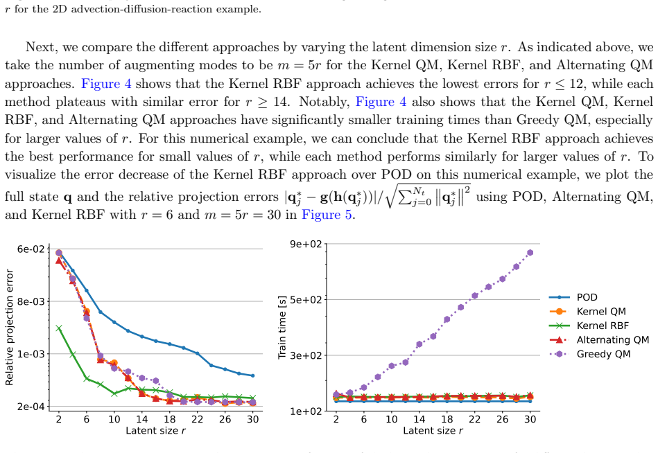
- On problems with slowly decaying Kolmogorov n-width, RBF-kernel manifolds can reach target projection accuracy at smaller latent dimension than POD or quadratic manifolds, which would make downstream reduced-order models cheaper to evaluate.
- For very hard problems, such as the double Mach reflection test, nonlinear augmentation yields only slight improvement over POD because these manifolds still inherit the limits of their underlying linear basis.
Reading between the lines
- The same kernel correction map could be embedded in time-stepping reduced-order models to close the modal equations during online simulation; the paper lists this as future work and does not demonstrate it.
- A parameterized or multi-task kernel that shares information across parameter values might improve transfer to unseen parameters; the paper trains one kernel interpolant on pooled snapshots, which is a cruder form of sharing.
- Because the exact low-to-high mode map is not well-defined, the correction's value is inherently about average projection quality rather than recovering discarded modes individually; future theory could target expected-error bounds instead of pointwise map estimates.
- A practical test of the method's robustness would be to fix kernel and regularization choices on a training-only validation split, then check whether the reported accuracy ordering across latent dimensions persists on a new parameter value.
Editorial analysis
A structured set of objections, weighed in public.
Referee Report
Summary. The paper introduces 'kernel manifold' (KM) dimensionality reduction, a nonlinear-augmentation method that augments a POD decoder with a correction term n(bq) learned by regularized kernel interpolation in a reproducing kernel Hilbert space. The decoder has the form g(bq) = qbar + V bq + V n(bq), where n solves (K(bQ,bQ)+lambda I)Omega = bP^T. The authors show that the feature-map/quadratic-manifold formulation and the GP/RBF closure of [10] are special cases, and they report numerical comparisons against POD, Alternating QM, and Greedy QM on four test problems: advection-diffusion-reaction, an analytic surface-heating model, a 3D hyperelastic bracket, and double Mach reflection. The central mathematical derivation in Sections 3.1-3.3 is sound: the reduction of (3.5) to (3.7) is a valid orthogonality argument, and the Representer Theorem is applied correctly. The main weakness is empirical: the hyperparameters used in the reported error curves are selected using the same test data on which the methods are then evaluated, so the headline accuracy comparisons are optimistically biased.
Significance. If the empirical claims survive a clean validation protocol, this is a useful and reasonably general contribution. The unification of feature-map manifolds and RBF/GP closures within one RKHS framework is natural and clearly explained, and the method has a genuine practical advantage when high-order polynomial feature maps would make the FM normal equations large: the KM linear system (3.9) scales with the number of snapshots rather than the feature dimension. The derivation is machine-checkable in spirit and the special cases are shown honestly rather than assumed. The paper also reports a fair range of negative results (e.g., double Mach reflection, where nonlinear augmentation gives only marginal gains), which strengthens credibility. The main obstacle is that the numerical support for the central accuracy claim is contaminated by test-set hyperparameter tuning in Appendix A, and the abstract's monotonicity claim is unproved and imprecise. With a corrected validation protocol and a clarified monotonicity statement, the paper would be a solid contribution to nonlinear model reduction.
major comments (2)
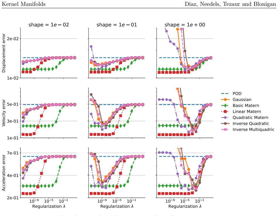
- [Appendix A and Section 4] Hyperparameters are selected on the same test data later used for the headline error curves. In A.1 the RBF kernel and shape are chosen as the 'lowest error' on the alpha=1e-3 test set (Fig. 24); A.2 chooses Gaussian/epsilon=1e-1 from Fig. 26; A.3 chooses linear Matern from Fig. 28; A.4 chooses inverse quadratic/epsilon=1e-3 from Fig. 30. Regularization values for all methods, including baselines, are fixed from test-error sweeps in Figs. 25, 27, 29, and 31 and reported in Tables 2-5. The comparisons in Figs. 4, 9, 15, and 22 therefore report test-informed tuning performance, not unbiased out-of-sample generalization, and the KM gains over QM/POD are likely optimistic. Please re-run the comparison with a validation split (or nested CV) for hyperparameter selection and reserve the test set for final evaluation; if that is infeasible, state the protocol explicitly and label the reported er
- [Abstract and Section 3.2] The claim that KM error decreases monotonically as the latent dimension increases is stated without proof or formalization. In the decoder (3.10), when r increases by one and m is fixed, V and V both change: the first column of the old V becomes a linear mode and the last augmenting mode is dropped from the correction. The feasible sets in (3.5) are therefore not nested, so monotonicity of the projection error in r is not automatic. If the intended statement is monotonicity in m, it should be stated as a property of the training objective (larger codomain with fixed lambda) and distinguished from test projection error. Please either prove the intended statement for the appropriate variable or remove/qualify the claim.
minor comments (5)
- [Section 4.3] The text says 'Table 3 lists the regularization values' but the table is numbered Table 4.
- [Section 4.1] 'scipy.interpolate.solve ivp()' should be 'scipy.integrate.solve_ivp()'.
- [Section 3.3, Eq. (3.16)] The grouping Omega^T phi(bQ)^T G is dimensionally sensible but would benefit from an explicit dimension statement; the notation is easy to misread as Omega^T (phi(bQ)^T G phi(bq)) rather than (Omega^T phi(bQ)^T G) phi(bq).
- [Section 4.3 / Figure 14] The statement 'Kernel RBF has monotonically decreasing error as m increases' is made for this example; given the abstract's stronger global claim, please clarify here that this is an empirical observation rather than a consequence of the method.
- [Section 5] Typo: 'autencoders' should be 'autoencoders'.
Circularity Check
Core RKHS derivation is self-contained; no circular derivation steps. Empirical comparisons are weakened by test-set hyperparameter selection, but that is a validation flaw rather than derivation circularity.
full rationale
The derivation in Sections 3.1–3.3 is self-contained: the KM decoder (3.10) solves the regularized least-squares problem (3.5)/(3.7) in an RKHS, and the Representer Theorem (Theorem 3.1) directly yields the finite-dimensional solution n(bq) = Omega^T K(bQ,bq) with (K(bQ,bQ)+lambda I)Omega = bP^T. No quantity in this derivation is defined in terms of the reported test errors, and the equivalence of feature-map kernels to FM/QM decoders (3.15)–(3.17) and of RBF kernels to the GP/RBF closure (Remark 3.2) is shown by explicit construction, not assumed. The self-citations [10] and [12] are contextual and not load-bearing: [10] is used only in Remark 3.2 to state an equivalence that follows from the same Representer Theorem, and [12] is mentioned as future work. The main caveat is empirical: Appendix A selects the RBF kernel, shape parameter, and regularization by minimizing testing error (e.g., A.1: 'Among the combinations tested, the quadratic Matérn kernel with shape ϵ = 10−2 achieved the lowest error of E = 5.07 × 10⁻⁴ at regularization λ = 10−10. Therefore, we use the quadratic Matérn kernel...'), and Section 4 reuses those settings to report test errors. This is test-set leakage that makes the headline accuracy gains optimistic and can bias method comparisons, but it does not make the mathematical derivation circular. Remark 2.3 also honestly notes the exact map n* is not well-defined and no generalization bounds are supplied, so the empirical demonstration is the main support for the central accuracy claim and that support is contaminated by the Appendix A protocol. These are correctness/validation concerns, not definitional circularity.
Assumptions & free parameters
free parameters (5)
- RBF shape parameter epsilon =
1e-2 (advection-diffusion-reaction), 1e-1 (surface heating), 1e-1 (bracket), 1e-3 (Euler)
- Regularization parameter lambda =
Varies per method and problem, e.g., Kernel RBF lambda=1e-11, 1e-9, 1e-7, 1e-3 in the four examples
- Kernel choice =
Quadratic Matérn, Gaussian, linear Matérn, inverse quadratic across examples
- Number of augmenting modes m =
Set to 5r, 10r, 4r depending on example
- Input normalization setting =
Applied in some examples, not in others
assumptions (5)
- standard math Representer Theorem (Theorem 3.1): minimizer of (3.2) has form s(x)=Omega^T K(X,x) and solves (K+lambda I)Omega = Y^T
- standard math Moore-Aronszajn theorem: each positive-definite kernel defines a unique RKHS
- standard math Orthonormality and complementarity of POD mode matrices V and Vbar (V^T V = I_r, Vbar^T Vbar = I_m, V^T Vbar = 0)
- domain assumption The map from low-order modal coefficients bq to high-order modal coefficients bp is learnable as an RKHS function that generalizes out-of-sample
- domain assumption Training data is representative of the test distribution in the sense that kernel interpolation of bq to bp transfers
Cite this review
Pith. "Pith review of Kernel manifolds: nonlinear-augmentation dimensionality reduction using reproducing kernel Hilbert spaces." pith.science (2026). https://pith.science/paper/UL5TR2TO
@misc{pith2026250900224,
  author       = {Pith},
  title        = {Pith review of: Kernel manifolds: nonlinear-augmentation dimensionality reduction using reproducing kernel Hilbert spaces},
  year         = {2026},
  howpublished = {\url{https://pith.science/paper/UL5TR2TO}},
  note         = {Machine review of arXiv:2509.00224}
}
read the original abstract
This paper generalizes recent advances on quadratic manifold (QM) dimensionality reduction by developing kernel methods-based nonlinear-augmentation dimensionality reduction. QMs, and more generally feature map-based nonlinear corrections, augment linear dimensionality reduction with a nonlinear correction term in the reconstruction map to overcome approximation accuracy limitations of purely linear approaches. While feature map-based approaches typically learn a least-squares optimal polynomial correction term, we generalize this approach by learning an optimal nonlinear correction from a user-defined reproducing kernel Hilbert space. Our approach allows one to impose arbitrary nonlinear structure on the correction term, including polynomial structure, and includes feature map and radial basis function-based corrections as special cases. Furthermore, our method has relatively low training cost and has monotonically decreasing error as the latent space dimension increases. We compare our approach to proper orthogonal decomposition and several recent QM approaches on data from several example problems.
Figures


Figures from the paper (28 more)




Forward citations
Cited by 1 Pith paper
-
Hybrid coupling with operator inference and the overlapping Schwarz alternating method
Overlapping Schwarz iteration can glue operator-inference ROMs to each other and to full-order finite-element models for 3D nonlinear solid dynamics, with online speedups up to 106x.
Reference graph
Works this paper leans on
- [10]
- [1]
-
[2]
P. J. Baddoo, B. Herrmann, B. J. McKeon, and S. L. Brunton. Kernel learning for robust dynamic mode decomposition: linear and nonlinear disambiguation optimization. Proceedings of the Royal Society A , 478(2260):20210830, 2022
work page 2022
-
[3]
J. Barnett and C. Farhat. Quadratic approximation manifold for mitigating the kolmogorov barrier in nonlinear projection-based model order reduction. Journal of Computational Physics , 464:111348, 2022
work page 2022
-
[4]
J. Barnett, C. Farhat, and Y. Maday. Neural-network-augmented projection-based model order reduc- tion for mitigating the Kolmogorov barrier to reducibility. J. Comput. Phys. , 492:Paper No. 112420, 20, 2023
work page 2023
- [5]
- [6]
-
[7]
C. Bonneville, Y. Choi, D. Ghosh, and J. L. Belof. Gplasdi: Gaussian process-based interpretable latent space dynamics identification through deep autoencoder. Computer Methods in Applied Mechanics and Engineering, 418:116535, 2024
work page 2024
Show all 48 references
-
[8]
Bonneville, X
C. Bonneville, X. He, A. Tran, J. S. Park, W. Fries, D. A. Messenger, S. W. Cheung, Y. Shin, D. M. Bortz, D. Ghosh, J.-S. Chen, J. Belof, and Y. Choi. A comprehensive review of latent space dynam- ics identification algorithms for intrusive and non-intrusive reduced-order-mode...
2024 arXiv
-
[9]
Cocola, J
J. Cocola, J. Tencer, F. Rizzi, E. Parish, and P. Blonigan. Hyper-reduced autoencoders for efficient and accurate nonlinear model reductions, 2023
2023
-
[11]
A. N. Diaz, Y. Choi, and M. Heinkenschloss. A fast and accurate domain-decomposition nonlinear manifold reduced order model. Comput. Methods Appl. Mech. Engrg. , 425:116943, 2024
2024
-
[12]
A. N. Diaz, S. A. McQuarrie, J. T. Tencer, and P. J. Blonigan. Interpretable and flexible non-intrusive reduced-order models using reproducing kernel hilbert spaces. arXiv preprint arXiv:2506.10224 , 2025
2025
-
[13]
W. D. Fries, X. He, and Y. Choi. Lasdi: Parametric latent space dynamics identification. Computer Methods in Applied Mechanics and Engineering , 399:115436, 2022
2022
-
[14]
Geelen, L
R. Geelen, L. Balzano, S. Wright, and K. Willcox. Learning physics-based reduced-order models from data using nonlinear manifolds. Chaos: An Interdisciplinary Journal of Nonlinear Science, 34(3):033122, 03 2024
2024
-
[15]
Geelen, S
R. Geelen, S. Wright, and K. Willcox. Operator inference for non-intrusive model reduction with quadratic manifolds. Computer Methods in Applied Mechanics and Engineering , 403:115717, 2023
2023
-
[16]
Ghattas and K
O. Ghattas and K. Willcox. Learning physics-based models from data: Perspectives from inverse problems and model reduction. Acta Numerica, 30:445–554, 2021
2021
-
[17]
Goyal and P
P. Goyal and P. Benner. Generalized quadratic embeddings for nonlinear dynamics using deep learning. Physica D: Nonlinear Phenomena , 463:134158, 2024
2024
-
[18]
Gruber and I
A. Gruber and I. Tezaur. Variationally consistent hamiltonian model reduction. SIAM Journal on Applied Dynamical Systems , 24(1):376–414, 2025
2025
-
[19]
Gubisch and S
M. Gubisch and S. Volkwein. Chapter 1: Proper Orthogonal Decomposition for linear-quadratic optimal control. In P. Benner, A. Cohen, M. Ohlberger, and K. Willcox, editors, Model Reduction and Approx- imation: Theory and Algorithms , Computational Science and Engineering, pages...
-
[20]
M. D. Gunzburger, J. S. Peterson, and J. N. Shadid. Reduced-order modeling of time-dependent pdes with multiple parameters in the boundary data. Computer Methods in Applied Mechanics and Engineering, 196(4):1030–1047, 2007
2007
-
[21]
Hinze and S
M. Hinze and S. Volkwein. Proper orthogonal decomposition surrogate models for nonlinear dynamical systems: Error estimates and suboptimal control. In P. Benner, V. Mehrmann, and D. C. Sorensen, editors, Dimension Reduction of Large-Scale Systems , Lecture Notes in Computation...
2005
-
[22]
S. Jain, P. Tiso, J. B. Rutzmoser, and D. J. Rixen. A quadratic manifold for model order reduction of nonlinear structural dynamics. Computers & Structures , 188:80–94, 2017
2017
-
[23]
Jalalian, J
Y. Jalalian, J. F. O. Ramirez, A. Hsu, B. Hosseini, and H. Owhadi. Data-efficient kernel methods for learning differential equations and their solution operators: Algorithms and error analysis. arXiv preprint arXiv:2503.01036, 2025
2025 arXiv
-
[24]
Y. Kim, Y. Choi, D. Widemann, and T. Zohdi. A fast and accurate physics-informed neural network reduced order model with shallow masked autoencoder. Journal of Computational Physics , 451:Paper No. 110841, 29, 2022
2022
-
[25]
Kramer, B
B. Kramer, B. Peherstorfer, and K. Willcox. Learning nonlinear reduced models from data with operator inference. Annual Review of Fluid Mechanics , 56:521–548, 2024
2024
-
[26]
Lance, A
B. Lance, A. M. Krueger, B. A. Freno, and R. M. Wagnild. Validation Study of the Multi-Fidelity Toolkit. 2022
2022
-
[27]
B. W. Larsen, T. G. Kolda, A. R. Zhang, and A. H. Williams. Tensor decomposition meets rkhs: Efficient algorithms for smooth and misaligned data. arXiv preprint arXiv:2408.05677 , 2024
2024 arXiv
-
[28]
Lee and K
K. Lee and K. T. Carlberg. Model reduction of dynamical systems on nonlinear manifolds using deep convolutional autoencoders. Journal of Computational Physics , 404:108973, 32, 2020
2020
-
[29]
Lowery, J
M. Lowery, J. Turnage, Z. Morrow, J. D. Jakeman, A. Narayan, S. Zhe, and V. Shankar. Kernel neural operators (knos) for scalable, memory-efficient, geometrically-flexible operator learning. arXiv preprint arXiv:2407.00809, 2024
2024 arXiv
-
[30]
C. A. Micchelli and M. Pontil. On learning vector-valued functions. Neural computation, 17(1):177–204, 2005
2005
-
[31]
Mota and J
A. Mota and J. A. Zimmerman. A variational, finite-deformation constitutive model for piezoelectric materials. International Journal for Numerical Methods in Engineering , 85(6):752–767, 2011
2011
-
[32]
Ohlberger and S
M. Ohlberger and S. Rave. Reduced basis methods: Success, limitations and future challenges. Pro- ceedings of the Conference Algoritmy , pages 1–12, 2016
2016
-
[33]
Parish, M
E. Parish, M. Yano, I. Tezaur, and T. Iliescu. Residual-based stabilized reduced-order models of the transient convection–diffusion–reaction equation obtained through discrete and continuous projection. Archives of Computational Methods in Engineering , 32:1885–1929, 2025
1929
-
[34]
Peherstorfer and K
B. Peherstorfer and K. Willcox. Data-driven operator inference for nonintrusive projection-based model reduction. Comput. Methods Appl. Mech. Engrg. , 306:196–215, 2016
2016
-
[35]
E. Qian, B. Kramer, B. Peherstorfer, and K. Willcox. Lift & learn: Physics-informed machine learning for large-scale nonlinear dynamical systems. Physica D: Nonlinear Phenomena , 406:132401, 2020
2020
-
[36]
Romor, G
F. Romor, G. Stabile, and G. Rozza. Non-linear manifold reduced-order models with convolutional autoencoders and reduced over-collocation method. Journal of Scientific Computing , 94(3):Paper No. 74, 2023
2023
-
[37]
J. B. Rutzmoser, D. J. Rixen, P. Tiso, and S. Jain. Generalization of quadratic manifolds for reduced order modeling of nonlinear structural dynamics. Computers & Structures , 192:196–209, 2017
2017
-
[38]
Salvador, L
M. Salvador, L. Dede, and A. Manzoni. Non intrusive reduced order modeling of parametrized pdes by kernel pod and neural networks. Computers & Mathematics with Applications , 104:1–13, 2021. 35 Kernel Manifolds Diaz, Needels, Tezaur and Blonigan
2021
-
[39]
G. Santin. Approximation with kernel methods, 2018. Lecture Notes WS 2017/18, Department of Mathematics, University Stuttgart, Germany
2018
-
[40]
Santin and B
G. Santin and B. Haasdonk. 9 kernel methods for surrogate modeling. In P. Benner, S. Grivet-Talocia, A. Quarteroni, G. Rozza, W. Schilders, and L. M. Silveira, editors, Model Order Reduction. Volume 1: System- and Data-Driven Methods and Algorithms , pages 311–354. Walter de G...
2021
-
[41]
Sch¨ olkopf, A
B. Sch¨ olkopf, A. Smola, and K.-R. M¨ uller. Kernel principal component analysis. In International conference on artificial neural networks , pages 583–588. Springer, 1997
1997
-
[42]
Schwerdtner, P
P. Schwerdtner, P. Mohan, A. Pachalieva, J. Bessac, D. O’Malley, and B. Peherstorfer. Online learning of quadratic manifolds from streaming data for nonlinear dimensionality reduction and nonlinear model reduction. Proceedings of the Royal Society A , 481(2314):20240670, 2025
2025
-
[43]
Schwerdtner and B
P. Schwerdtner and B. Peherstorfer. Greedy construction of quadratic manifolds for nonlinear dimen- sionality reduction and nonlinear model reduction. arXiv preprint arXiv:2403.06732 , 2024
2024 arXiv
-
[44]
L. F. Shampine and M. W. Reichelt. The MATLAB ODE suite. SIAM Journal on Scientific Computing , 18(1):1–22, 1997
1997
-
[45]
Virtanen, R
P. Virtanen, R. Gommers, T. E. Oliphant, M. Haberland, T. Reddy, D. Cournapeau, E. Burovski, P. Peterson, W. Weckesser, J. Bright, S. J. van der Walt, M. Brett, J. Wilson, K. J. Millman, N. Mayorov, A. R. J. Nelson, E. Jones, R. Kern, E. Larson, C. J. Carey,˙I. Polat, Y. Feng,...
2020
-
[46]
Wendland
H. Wendland. Scattered data approximation, volume 17. Cambridge university press, 2004
2004
-
[47]
Woodward and P
P. Woodward and P. Colella. The numerical simulation of two-dimensional fluid flow with strong shocks. Journal of computational physics , 54(1):115–173, 1984
1984
-
[48]
G. B. Wright. Radial basis function interpolation: numerical and analytical developments . University of Colorado at Boulder, 2003. 36
2003
Reviewed August 5, 2026 · model on record in the stance chip above.
Discussion (0). Continue with ORCID to comment.