Bridge the Inference Gaps of Neural Processes via Expectation Maximization

Herke van Hoof; Marco Federici; Qi Wang

REVIEW 2 major objections 5 minor 1 cited by

Bridge the Inference Gaps of Neural Processes via Expectation Maximization

T0 review · 2 major / 5 minor · reviewed 2026-08-10 · deepseek-v4-flash

Challenge this review Re-run · record.json Download PDF Read on arXiv ↗ Review JSON

Pith's one-line read Neural processes underfit because their training objective is an invalid ELBO, and a variational-EM surrogate with self-normalized importance sampling is proven to increase the true log-likelihood to a local optimum.

desk verdict Useful NP objective and a correct diagnosis of the vanilla NP's invalid ELBO, but the advertised log-likelihood improvement guarantee only holds for the exact EM surrogate, not the biased finite-particle SNIS algorithm they actually run. read the letter →

arxiv 2501.03264 v1 pith:YH2VTQJP submitted 2025-01-04 cs.LG cs.AIcs.NE

Qi Wang , Marco Federici , Herke van Hoof This is my paper · ORCID

classification cs.LGcs.AIcs.NE

keywords neuralprocessesexpectationmaximizationself-normalizedimportancesamplingfunctionalpriorvariationalinferencemeta-learningcollapse

verification ladder T0 review T1 audit T2 compute T3 formal

The pith

A machine-rendered reading of the paper's core claim, the machinery that carries it, and where it could break.

The reading

The paper argues that neural processes underfit because their training objective is an invalid ELBO (evidence lower bound), not because the model family is weak. It shows that the standard NP objective — a generative-likelihood term minus a KL divergence between an approximate posterior and an approximate prior — carries a 'prior approximation gap' of unknown sign, so maximizing it can push the true meta-dataset log-likelihood down. The fix is a variational expectation-maximization surrogate whose E-step averages against the exact posterior and whose M-step maximizes the joint log-likelihood; optimizing this surrogate by alternating steps is proven to increase the true log-likelihood monotonically and to reach at least a local optimum. Because the exact posterior average is intractable, the paper approximates it with self-normalized importance sampling, yielding the SI-NP objective it actually trains. If the guarantee holds, practitioners get an architecture-agnostic objective that improves on NP, CNP, and ML-NP baselines across synthetic regression, image completion, and Sim2Real benchmarks.

What carries the argument

The carrying object is the variational-EM surrogate function $L(\vartheta; \vartheta_k)$ of Eq. (10), a minorize-maximization surrogate of the meta-dataset log-likelihood: it is everywhere below $L(\vartheta)$ and touches it at $\vartheta = \vartheta_k$, so every M-step that improves the surrogate cannot decrease the true log-likelihood. What makes it tractable is the replacement of its posterior expectation by the self-normalized importance-sampling estimator in Eq. (12), where latent particles $z^{(b)}$ are drawn from a proposal $q_\eta(z|D_T)$ and weighted by normalized weights $\hat{\omega}^{(b)}$ proportional to $p(D_T|z^{(b)}; \vartheta_k) p(z^{(b)}|D_C; \vartheta_k) / q_\eta(z^{(b)}|D_T)$; these weights reallocate gradient toward particles that explain the target data well, which is the mechanism by which the functional prior adapts.

What would settle it

On a low-dimensional latent space, run Algorithm 1 with its default small particle budget (8 for image completion) and, after every EM iteration, evaluate the exact meta-dataset log-likelihood by numerical integration or an orders-of-magnitude larger particle count; any consecutive pair of iterations in which the exact log-likelihood decreases falsifies the improvement guarantee as implemented.

Watch

Extended reading notes

Core claim

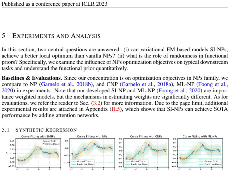
The paper's central claim is that the vanilla NP objective $L_{\mathrm{NP}}(\vartheta, \phi) = \mathbb{E}_{q_\phi(z)}[\ln p(D_T|z; \vartheta)] - D_{\mathrm{KL}}(q_\phi(z) \| q_\phi(z|D_C))$ is not a valid lower bound on the meta-dataset log-likelihood $L(\vartheta) = \ln p(D_T|D_C; \vartheta)$: substituting the approximate prior $q_\phi(z|D_C)$ for the learned functional prior $p(z|D_C; \vartheta)$ adds a prior-approximation gap of undetermined sign, so optimizing this 'consistent regularizer' can move the true objective the wrong way. In its place, the paper constructs the surrogate $L(\vartheta; \vartheta_k) = \mathbb{E}_{p(z|D_T;\vartheta_k)}[\ln p(D_T, z|D_C; \vartheta) - \ln p(z|D_T; \vartheta_k)]$, proves it minorizes the log-likelihood, and shows the EM update $\vartheta_{k+1} = \arg\max_\vartheta L(\vartheta; \vartheta_k)$ gives $L(\vartheta_{k+1}) \ge L(\vartheta_k)$ with convergence to at least a local optimum (Propositions 1-2). The tractable version replaces the intractable posterior expectation with a self-normalized importance-sampling estimate over particles $z^{(b)}$ drawn from a proposal $q_\eta(z|D_T)$, defaulting to the functional prior as the proposal; with one particle, the objective collapses the functional prior to a Dirac delta, making SI-NP exactly CNP (Proposition 3). The paper reports that SI-NP outperforms NP, CNP, and ML-NP objectives on GP-kernel regression, image completion, and Sim2Real benchmarks, with attention-augmented SI-ANP reaching the best results among the compared baselines.

Load-bearing premise

The monotone-improvement guarantee is proved for the exact posterior expectation, while the implemented algorithm replaces that expectation with a self-normalized importance-sampling estimate using 8 or 16 particles; the guarantee transfers to the implemented method only if that finite-particle bias is negligible.

Editorial extensions

If this is right

The same encoder-decoder architectures used by NP, CNP, and ML-NP can be kept unchanged; switching to the SI-NP objective is what aligns training with the meta-dataset log-likelihood, so the gain is orthogonal to architecture and compounds with structural inductive biases.
With one Monte Carlo particle, SI-NP provably collapses to CNP, which explains why deterministic conditional models are competitive on simple tasks while multi-particle SI-NP retains functional-prior uncertainty on complex tasks.
Because SI-NP is an importance-weighted objective, its evaluation log-likelihood rises with the number of particles, so the 32-particle numbers reported are lower bounds on its performance in the particle limit.
The learned functional prior's covariance trace tracks the semantic complexity of the task family and shrinks as context points grow, giving a quantitative diagnostic for when latent randomness matters.

Reading between the lines

Editorial extensions of the paper, not claims the author makes directly.

A direct test of the guarantee would track the exact (large-particle) meta-dataset log-likelihood across EM iterations with B = 8 or 16; if it ever decreases, the implemented finite-sample objective, not the exact surrogate, is what fails to satisfy Proposition 2.
The optional proposal update (E-step #2) was skipped because joint training was unstable; finding a stable schedule for it is the most promising route to larger effective sample sizes and a tighter match between the implemented objective and the proven surrogate.
Because the objective is architecture-agnostic, the same EM surrogate could be ported to other learned-prior stochastic-process models such as deep Gaussian processes, where the same invalid-ELBO diagnosis would apply.
The empirically observed prior collapse on MNIST suggests a regime map: on low-semantic-complexity tasks SI-NP will behave like a deterministic CNP, so the multi-particle objective is primarily buying performance where function families are semantically rich.

Share X Bluesky LinkedIn Reddit HN

Editorial analysis

A structured set of objections, weighed in public.

Desk editor's note, referee report, and a circularity audit.

Desk Editor's Note

read the letter

Read this paper. The useful part is the diagnosis: the vanilla NP objective is not a valid ELBO. They show the KL term compares the approximate posterior to a learned approximate prior, and the gap to the true functional prior has an unknown sign, so optimizing it has no guaranteed relationship to the marginal log-likelihood. That alone is worth a citation for people working on NP objectives. The proposed fix, SI-NP, wraps EM around a self-normalized importance sampling objective and is a sensible extension of reweighted wake-sleep to learned-functional-prior settings. The one-sample equivalence with CNP (Proposition 3) is a nice observation, and their experiments show consistent, if modest, improvements over NP/CNP/ML-NP across synthetic and image benchmarks. They release code and are reasonably open about limitations.

The soft spot is the central theoretical claim. Proposition 2 gives a genuine improvement guarantee, but it is proved for the exact posterior EM surrogate in Eq. (10). The implemented Algorithm 1 replaces the posterior with self-normalized importance sampling using the functional prior as proposal, with B=8 or 16 particles, and the optional proposal update is skipped. SNIS is biased at finite B and no finite-B bound is supplied; the paper only cites asymptotic consistency. So the monotone-improvement claim does not cover the method as trained. This is an overclaim in the abstract, even though the appendix does acknowledge the bias. A revision should rephrase the guarantee as asymptotic (or for the exact EM iterations) and preferably add a finite-B analysis or at least a diagnostic. Secondary issue: the proof of Proposition 3 in Appendix F.1 is suspect. Because z is reparameterized as mu + epsilon sigma, the term (mu - zhat)^2/sigma^2 is O(1), not kappa/sigma^2 with fixed kappa, so the L'Hopital computation looks misapplied. The conclusion that the prior collapses at one sample may still be true via the -ln sigma term, but the written proof needs correction.

For a reader, the paper delivers: the invalid-ELBO diagnosis is new and useful, the objective is a reasonable competitor, and the experiments support the qualitative claims. The guarantee gap is real but not disqualifying if the claims are softened. I would send this to peer review; it deserves a serious referee who insists on fixing the Proposition 3 proof and rephrasing the guarantee. Bring it to reading group if your group does meta-learning or variational inference.

Referee Report

2 major / 5 minor

Summary. The paper studies neural processes (NPs) from the perspective of the optimization objective. It argues that the standard NP approximate ELBO, which uses an approximate functional prior in the KL regularizer, is not a valid variational objective and can fail to improve the marginal log-likelihood. The authors propose SI-NP, a training objective derived from a variational expectation-maximization surrogate of the meta-dataset log-likelihood. In the exact formulation, the E-step uses the posterior under the current parameters and the M-step maximizes an expected joint log-likelihood; Propositions 1 and 2 claim that this exact EM procedure is a surrogate with a monotonic improvement guarantee. Since the exact posterior is intractable, the implemented algorithm uses self-normalized importance sampling with the functional prior as the proposal, with B=8 or 16 particles. The paper reports experiments on synthetic GP regression, image completion, and Sim2Real benchmarks, finding that SI-NP is competitive with or better than NP, CNP, and ML-NP, with additional gains when augmented with attention. The paper also includes a one-sample analysis (Proposition 3) claiming equivalence of SI-NP with CNP via prior collapse, and extensive appendix ablations.

Significance. If the theoretical guarantee held for the implemented algorithm, this would be a valuable contribution: it would place NP training on a principled EM footing, connect one-sample SI-NP to CNP, and explain observed underfitting of vanilla NPs. The exact-surrogate EM derivation is standard and correct, and the paper ships code plus extensive ablations over particle count, latent dimension, and attention augmentation, which strengthen the empirical story. The empirical results are credible and show consistent gains across multiple benchmarks. However, the advertised improvement guarantee is proved only for the exact EM surrogate, whereas the objective actually optimized is a finite-B self-normalized importance sampling estimate that is biased and is not a lower bound on the target log-likelihood. This gap is load-bearing for the paper's central theoretical claim, so the significance of the theoretical contribution is contingent on either repairing the analysis or substantially qualifying the claim.

major comments (2)

[§4.1.2, Eq. (12), Algorithm 1, and §4.2] Proposition 2 proves monotonic improvement of the meta-dataset log-likelihood for the exact surrogate in Eq. (10), where the E-step uses the exact posterior p(z|DT;ϑ_k) and the M-step maximizes the exact expectation in Eq. (11). The implemented SI-NP instead maximizes the self-normalized importance sampling estimate in Eq. (12) with B=8 or 16 particles, using the functional prior as the proposal and skipping the optional proposal update (Algorithm 1, lines 2-8; §4.2). For finite B, SNIS is biased and is not a lower bound on the log-likelihood, so the guarantee of Proposition 2 does not transfer to the objective actually optimized. The only mitigation offered is asymptotic consistency (Appendix A, citing Owen 2013, Ch. 9), which does not establish monotonic improvement at finite B. The sentence in §4.2 that the method can 'theoretically find at least a local optimal' based on Proposition 2 is therefore too strong. Please either prove a finite-B bias bound or a monotonicity statement, or add training-time measurements of the true log-likelihood showing that L(ϑ_k) is non-decreasing in the implemented setting, and qualify Proposition 2 accordingly.
[Appendix F.1, Proof of Proposition 3] The proof of prior collapse for B=1 is not correct as written. In Eqs. (35)-(36) the sample is reparameterized as \hat z_i = μ_i + ε_i σ_i, so the quantity (μ_i - \hat z_i)^2/(2σ_i^2) equals ε_i^2/2 and is not of the form κ_i/σ_i^2 with κ_i independent of σ_i. The L'Hôpital calculation in Eq. (37) treats κ_i as σ-independent and applies L'Hôpital's rule to a ratio whose numerator tends to κ_i rather than to zero; for κ_i>0 the displayed limit is -∞, not +∞. The conclusion of Proposition 3 may still be true under a correctly specified argument in which the M-step optimizes a fixed sample from the old prior, but the derivation as presented does not establish it. Please rewrite the proof with an explicit distinction between the sampling distribution (old parameters) and the optimized parameters, and correct the limit analysis.

minor comments (5)

[Algorithm 1, line 2] The phrase 'reset the variational posterior q_ϕ(z) = p(z|DT;ϑ_k)' is misleading because this posterior is intractable and the implemented algorithm never constructs q_ϕ; the actual computation is the SNIS reweighting in Eq. (12). Please reword the algorithm description to make clear that the E-step is implemented by importance weighting rather than by exact posterior computation.
[Appendix F.1, Theorem 1] The result labeled 'L'Hôpital's Rule' is stated as an algebraic identity for differences rather than the standard rule for ratios; this makes the subsequent derivation hard to follow and should be rewritten.
[Appendix G.2 and Table 2] In the image completion experiments, the training particle count differs across methods (B=8 for SI-NP and B=16 for ML-NP). Please state explicitly whether the conclusions are robust to using the same B for all methods, or justify the asymmetric choice in the main text.
[General] There are several typographical and nomenclature issues: 'de Finneti' should be 'de Finetti' (Section 2), 'Marten' should be 'Matérn' throughout, and 'the the denominator' appears in Appendix E.3.1.
[Appendix H.1] The appendix reports that the learnable proposal update is unstable and that no results are shown for it, yet Algorithm 1 presents E-step #2 as an optional component of the method. Since all main experiments skip this step, the algorithm description should clearly mark the proposal update as a non-evaluated extension rather than part of the recommended procedure.

Circularity Check

0 steps flagged · score 0.0 of 10

No significant circularity; the EM surrogate and improvement guarantee follow from standard EM identities, self-citations are background, and the finite-B SNIS approximation gap is a correctness concern rather than a circular reduction.

full rationale

The derivation of the SI-NP objective is self-contained and non-circular. Equation (10) constructs the EM surrogate from the marginal log-likelihood in Eq. (4) by inserting the exact posterior and using the standard decomposition ln p(DT|DC;ϑ) = E_{p(z|DT;ϑ_k)}[ln p(DT,z|DC;ϑ) − ln p(z|DT;ϑ_k)] + KL[p(z|DT;ϑ_k) ∥ p(z|DT;ϑ)], so Proposition 2 and Appendix E.1.2 follow from nonnegativity of the KL term rather than from any assumption of the target result. The one-sample collapse result (Proposition 3, Appendix F.1) is a limit analysis of the stated SI-NP objective, and the claimed CNP equivalence is a derived consequence, not an input. The self-citations to Wang & van Hoof (2020, 2022) appear only in related-work and inductive-bias surveys; they are not used to justify the improvement guarantee or the empirical comparisons, and the benchmarks (GP simulators, MNIST/FMNIST/SVHN/CIFAR10, Lotka-Volterra) evaluate the method against independent external tasks. The skeptic's finite-B SNIS gap is real: Algorithm 1 optimizes a biased estimate of the exact EM surrogate, so the theoretical monotonicity guarantee is not automatically inherited by the implemented objective. That is a correctness or proof-transfer limitation, not a circular step, because the trained objective is an approximation of the same surrogate rather than a quantity defined in terms of the conclusion being claimed. Therefore no significant circularity is present.

Assumptions & free parameters 2 free parameters · 5 assumptions · 0 invented entities

The central claim rests on standard EM minorization theory, the exchangeable stochastic process assumption, diagonal Gaussian parameterization, and asymptotic consistency of self-normalized importance sampling. No new entities are invented. The key unaccounted quantity is the finite-B bias of the SNIS estimate, which is the gap between the proven EM guarantee and the implemented algorithm.

free parameters (2)

Number of SNIS particles B = 8 (image completion), 16 (synthetic regression)
Chosen by hand to balance computation and performance; the finite-B bias of self-normalized importance weights is not quantified and the improvement guarantee is asymptotic.
Latent dimension d = 128
Standard in prior NP work; Appendix H.3 reports negligible sensitivity across 32-256.

assumptions (5)

standard math The function L(ϑ;ϑ_k) in Eq. (10) is a valid minorizer of the marginal log-likelihood, satisfying g(ϑ;ϑ_k) ≤ f(ϑ) and g(ϑ_k;ϑ_k) = f(ϑ_k).
This is the standard EM/MM property used in Proposition 1 and Appendix E.1.1; it holds when the expectations are exact.
domain assumption The NP generative process defines an exchangeable stochastic process via Kolmogorov extension and de Finetti's theorem (Section 2, Eq. (1)).
The paper relies on this to justify the marginal likelihood objective of Eq. (3).
domain assumption The prior, posterior, and proposal distributions are diagonal Gaussians (Section 2, Preliminaries).
Used in Proposition 3 to prove one-sample prior collapse; the proof explicitly uses N(z; μ, diag(σ^2)).
standard math Self-normalized importance sampling estimates converge to the true expectation as B→∞ (Owen 2013), and the finite-B bias is negligible in practice.
This bridges the exact EM surrogate in Eq. (10) to the SNIS objective in Eq. (12); the paper acknowledges the finite-B bias but does not bound it.
domain assumption The approximate posterior family is flexible enough that the NP's 'consistent regularizer' (Eq. 7) is the source of suboptimality.
Remark 1 and Appendix D.2 analyze the prior approximation gap; the conclusion depends on the relationship between q_φ(z|D_C) and the true prior p(z|D_C;θ) being uncontrolled.

how reviews work

0 comments

Cite this review

Pith. "Pith review of Bridge the Inference Gaps of Neural Processes via Expectation Maximization." pith.science (2026). https://pith.science/paper/YH2VTQJP

@misc{pith2026250103264,
  author       = {Pith},
  title        = {Pith review of: Bridge the Inference Gaps of Neural Processes via Expectation Maximization},
  year         = {2026},
  howpublished = {\url{https://pith.science/paper/YH2VTQJP}},
  note         = {Machine review of arXiv:2501.03264}
}

read the original abstract

The neural process (NP) is a family of computationally efficient models for learning distributions over functions. However, it suffers from under-fitting and shows suboptimal performance in practice. Researchers have primarily focused on incorporating diverse structural inductive biases, \textit{e.g.} attention or convolution, in modeling. The topic of inference suboptimality and an analysis of the NP from the optimization objective perspective has hardly been studied in earlier work. To fix this issue, we propose a surrogate objective of the target log-likelihood of the meta dataset within the expectation maximization framework. The resulting model, referred to as the Self-normalized Importance weighted Neural Process (SI-NP), can learn a more accurate functional prior and has an improvement guarantee concerning the target log-likelihood. Experimental results show the competitive performance of SI-NP over other NPs objectives and illustrate that structural inductive biases, such as attention modules, can also augment our method to achieve SOTA performance. Our code is available at \url{https://github.com/hhq123gogogo/SI_NPs}.

Figures

Figures reproduced from arXiv: 2501.03264 by the authors.

**Figure 1.** Deep Latent Variable Models for Neural Processes. Here DC and DT respectively denote the context points for the functional prior inference and the target points for the function prediction. The global latent variable z is to summarize function properties. The model involves a functional prior distribution p(z|DC ; ϑ) and a functional generative distribution p(DT |z; ϑ). Please refer to Section (2) for detailed… view at source ↗

**Figure 2.** Illustration of Expectation Maximization for NPs. Green lines indicate the results after the E-steps while the red lines are for the M-steps in Algorithm (1). In the convergence iteration, the performance gap L(ϑH) − L(ϑH−1) is close to zero and the algorithm results in at least a local optimal solution. Values of these quantities are increased from the left to the right. 4.1 VARIATIONAL EXPECTATION MAXIMIZATION FOR… view at source ↗

**Figure 3.** Examples of Curve Fitting in RBF Kernel Cases. The plots report predictive mean functions with ±3 standard deviations. We create synthetic regression tasks by sampling functions from Gaussian processes. Three types of kernels, respectively Matern− 5 2 , RBF, and Periodic, are used to generate diverse function distributions. In each iteration, a batch of data points from functions is randomly processed into the cont… view at source ↗

Figures from the paper (20 more)

**Figure 4.** Figure 4: SI-NP Completed Images. From top to bottom in rows are original images, context points, learned predictive means and variances of sampled images. In the evaluation, the number of context pixels is randomly selected for each image in the dataset. We examine the perfor…

**Figure 5.** Figure 5: Asymptotic Performance in Image Completion. We meta test pixel average loglikelihoods with varying number of context points in image datasets. Context points are randomly selected for each image in testing processes. For MNIST/FMNIST datasets, the numbers of context p…

**Figure 6.** Figure 6: Statistics of Learned Functional Priors in ML-NPs/SI-NPs. In meta testing, we still vary the number of context points in image datasets. The trace of learned functional priors’ covariance matrices Tr[Σϑ(DC τ )] is computed based on p(z|DC τ ; ϑ) = N (z; µϑ(DC τ ), Σϑ(…

**Figure 7.** Figure 7: Computational Diagram of Vanilla NPs. The blue one and the pink one are, respectively, [PITH_FULL_IMAGE:figures/full_fig_p017_7.png]

**Figure 8.** Figure 8: Evaluation of Image Completion with Varying Number of Monte Carlo Particles. The [PITH_FULL_IMAGE:figures/full_fig_p027_8.png]

**Figure 9.** Figure 9: From the Left to the Right are population fitting results with [PITH_FULL_IMAGE:figures/full_fig_p027_9.png]

**Figure 10.** Figure 10: From the Left to the Right are population fitting results with [PITH_FULL_IMAGE:figures/full_fig_p029_10.png]

**Figure 11.** Figure 11: Examples of curve fitting in Marten kernel cases. [PITH_FULL_IMAGE:figures/full_fig_p030_11.png]

**Figure 12.** Figure 12: Examples of curve fitting in RBF kernel cases. [PITH_FULL_IMAGE:figures/full_fig_p030_12.png]

**Figure 13.** Figure 13: Examples of curve fitting in Periodic kernel cases. [PITH_FULL_IMAGE:figures/full_fig_p030_13.png]

**Figure 14.** Figure 14: Examples of Curve Fitting in Matern Kernel Cases. [PITH_FULL_IMAGE:figures/full_fig_p031_14.png]

**Figure 15.** Figure 15: Examples of Curve Fitting in RBF Kernel Cases. [PITH_FULL_IMAGE:figures/full_fig_p031_15.png]

**Figure 16.** Figure 16: Examples of Curve Fitting in Periodic Kernel Cases. [PITH_FULL_IMAGE:figures/full_fig_p031_16.png]

**Figure 17.** Figure 17: Evaluation of KL Divergence Terms in Vanilla NPs. In meta testing, we still [PITH_FULL_IMAGE:figures/full_fig_p032_17.png]

**Figure 18.** Figure 18: Examples of Image Completion Results using SI-NPs. From top to bottom in rows are [PITH_FULL_IMAGE:figures/full_fig_p032_18.png]

**Figure 19.** Figure 19: Examples of Image Completion Results using SI-NPs. From top to bottom in rows are [PITH_FULL_IMAGE:figures/full_fig_p033_19.png]

**Figure 20.** Figure 20: Examples of Image Completion Results using SI-NPs. From top to bottom in rows are [PITH_FULL_IMAGE:figures/full_fig_p033_20.png]

**Figure 21.** Figure 21: Examples of Image Completion Results using SI-NPs. From top to bottom in rows are [PITH_FULL_IMAGE:figures/full_fig_p033_21.png]

**Figure 22.** Figure 22: Examples of CIFAR10 Image Completion Results using SI-ANPs. From left to right and [PITH_FULL_IMAGE:figures/full_fig_p034_22.png]

**Figure 23.** Figure 23: Examples of FMNIST Image Completion Results using SI-ANPs. From left to right and [PITH_FULL_IMAGE:figures/full_fig_p034_23.png]

Discussion (0). Continue with ORCID to comment.

Forward citations

Cited by 1 Pith paper

Reviewed papers in the Pith corpus that reference this work. Sorted by Pith novelty score. Full citation record

Distance-informed Neural Processes
cs.LG 2025-08 conditional novelty 5.0 of 10

A neural process with a bi-Lipschitz-regularized local encoder achieves better uncertainty calibration and OOD detection than existing NP variants.

Reference graph

Works this paper leans on

27 extracted references · 22 canonical work pages · cited by 1 Pith paper

[1]

Vanilla NPs directly replace the real functional prior by the approximate one qϕ(z|DC τ ) and introduce the consistent regularizer in Eq. (7). We further introduce the prior approximation gap in Eq. (19), in which the sign is undetermined. LNP(ϑ, ϕ) = LELBO(ϑ, ϕ) + Eqϕ(z) ln qϕ(z|DC τ ) p(z|DCτ ; ϑ) | {z } Prior Approximation Gap (19) Based on decompositi...

work page 2015
[3]

Let z ∈ Rd be the latent variable for a diagonal Gaussian conditional prior p(z|DC τ ; ϑ) = N (z; µϑ(DC τ ), Σϑ(DC τ ))

Note that in our default setup of SI-NPs, the functional prior works as the proposal distribution to sample the latent variable. Let z ∈ Rd be the latent variable for a diagonal Gaussian conditional prior p(z|DC τ ; ϑ) = N (z; µϑ(DC τ ), Σϑ(DC τ )). Here the learned mean and the covariance matrix are simply denoted by µϑ = [µ1, . . . , µd]T ∈ Rd and Σϑ = ...

work page 2013
[4]

The training batch size for all images is 4 and we meta train the model until convergence (the maximum epoch number for MNIST/FMNIST is 100, and that for CIFAR10/SVHN is 200, and early stop is used when it reaches convergence). In meta training, the numbers of Monte Carlo samples are 16 for ML-NPs and 8 for SI-NPs (We find that 8 Monte Carlo samples are e...

work page 2019
[6]

Auto-encoding variational bayes

Diederik P Kingma and Max Welling. Auto-encoding variational bayes. arXiv preprint arXiv:1312.6114,

arXiv
[8]

11 Published as a conference paper at ICLR 2023 Art B. Owen. Monte carlo theory, methods and examples

work page 2023
[10]

3 3.2 Evaluation Criteria & Asymptotic Performance

12 Published as a conference paper at ICLR 2023 CONTENTS 1 Introduction 1 2 Preliminaries 2 3 Optimization Gaps and Statistical Traits 3 3.1 Inference Suboptimality in vanilla NPs . . . . . . . . . . . . . . . . . . . . . . . . 3 3.2 Evaluation Criteria & Asymptotic Performance . . . . . . . . . . . . . . . . . . . 4 4 Tractable Optimization via Expectati...

work page 2023
[12]

as an example. With context points DC = {(xi, yi)}n i=1 and target points DT = {(xi, yi)}n+m i=1 = [ xT , yT ], the key to applications is the predictive distribution p(f (xT )|DC, xT ) = N (yT ; µT , ΣT ). The conditional mean µT and covariance ΣT functions in Eq. (16) are permutation invariant to the order of context points. µT = mθ(xT ) + ΣT,C Σ−1 C,C ...

work page 2023
[13]

Prior Distribution

and works as a proxy for the non-analytical exact posterior p(z|DT τ ; ϑ). Prior Distribution. This is denoted by p(z|DC τ ; ϑ) in this paper. Unlike the approximate prior qϕ(z|DC τ ) used in NPs, we use an exact functional prior in SI-NPs. Proposal Distribution. This is denoted by qη(z|DT τ ) in this paper. The role of the proposal distri- bution resembl...

work page 2023

Show all 27 references

[15]

and more flexible prior distributions (Tomczak & Welling, 2018), to close VAEs inference gaps (Cremer et al.,

2018
[17]

Here we denote the approximate inference gap byDAI KL and the posterior approximation gap by DPA KL in Table (5)

to understand vanilla NPs. Here we denote the approximate inference gap byDAI KL and the posterior approximation gap by DPA KL in Table (5). Since it is infeasible to obtain the exact form for the functional posterior, we cannot directly close the mentioned approximate gap, an...

2023
[19]

To enable researchers to implement our developed method in studies, we leave the anonymous Github link here: https://anonymous.4open

except that the convolution modules are removed for the fair comparison since the inference objective is our research focus. To enable researchers to implement our developed method in studies, we leave the anonymous Github link here: https://anonymous.4open. science/r/SI_NPs-C...

2020
[21]

G.2 N EURAL ARCHITECTURES & OPTIMIZATIONS & E VALUATION SET-UP Synthetic Regression

for more details. G.2 N EURAL ARCHITECTURES & OPTIMIZATIONS & E VALUATION SET-UP Synthetic Regression. In terms of neural architectures, we use the same setup as that in (Gordon et al., 2019; Lee et al.,

2019
[23]

for more details. As in (Garnelo et al., 2018a), for theDecoder in all models, we use the modified standard deviation variable ˆσi = 0 .1 + 0.9 ∗ σi for the output distribution p(yi|xi, z; ϑ) in all benchmarks, where σi = MLPϑ(xi, zi). 25 Published as a conference paper at ICL...

2023
[24]

Our developed SI-NPs can be viewed as the conditional version of importance weighted autoen- coders, which explains the empirical observations in Fig

that LMC(ϑ; B1) ≥ LMC(ϑ; B2) with B1 ≥ B2. Our developed SI-NPs can be viewed as the conditional version of importance weighted autoen- coders, which explains the empirical observations in Fig. (8). However, when the prior is collapsed to a deterministic embedding, we do not e...

2023
[25]

To enable fair comparison, we also augment other baselines with attention networks

and compare the augmented one with other augmented baselines. To enable fair comparison, we also augment other baselines with attention networks. We apply the modification to all methods, and this operation results in ANP (Kim et al., 2019), ML-ANP and SI-ANPs. Neural Architec...

2019
[26]

We notice that the SI-ANP significantly beats other models in FMNIST/SVHN/CIFAR10 and is comparable with the ML-ANP in MNIST

0.985±0.019 1.062±0.019 0.574±0.023 LSI-ANP (ours) 0.995±0.017 1.071±0.017 0.56±0.024 H.5.2 I MAGE COMPLETION In Table (9), we report the results in image completion. We notice that the SI-ANP significantly beats other models in FMNIST/SVHN/CIFAR10 and is comparable with the M...

2023
[27]

For each run, we randomly sample 1000 functions as tasks to evaluate

in both context data points and target data points. For each run, we randomly sample 1000 functions as tasks to evaluate. # Sim (Lotka-V olterra) Real(Predator-Prey) LANP 2.211±0.017 -3.174±0.121 LML-ANP 2.203±0.042 -3.624±0.152 LSI-ANP (ours) 2.203±0.026 -2.822±0.316 In this ...

1935
[2006]

Reweighted wake-sleep

J¨org Bornschein and Yoshua Bengio. Reweighted wake-sleep. arXiv preprint arXiv:1406.2751 ,

arXiv
[2009]

and SVHN (Sermanet et al., 2012). In meta training and testing, we randomly select the number of context pixels n for each sampled batch of images (n ∼ U [1, 784] in MNIST/FMNIST and n ∼ U [1, 1023] in CIFAR10/SVHN). For pixel values, they are transformed to normalized Tensors...

2012
[2013]

Reweighted expectation maximization

Adji B Dieng and John Paisley. Reweighted expectation maximization. arXiv preprint arXiv:1906.05850,

1906 arXiv
[2015]

Factor analysis, probabilistic principal component analysis, variational inference, and variational autoencoder: Tutorial and survey

10 Published as a conference paper at ICLR 2023 Benyamin Ghojogh, Ali Ghodsi, Fakhri Karray, and Mark Crowley. Factor analysis, probabilistic principal component analysis, variational inference, and variational autoencoder: Tutorial and survey. arXiv preprint arXiv:2101.00734,

2023 arXiv
[2016]

Uncertainty in neural processes

Saeid Naderiparizi, Kenny Chiu, Benjamin Bloem-Reddy, and Frank Wood. Uncertainty in neural processes. arXiv preprint arXiv:2010.03753,

2010 arXiv
[2018]

In other words, the consistent regularizer in NPs is ill-posed for optimization

will not guarantee the performance improvement in a theoretical sense. In other words, the consistent regularizer in NPs is ill-posed for optimization. D.3 S UMMARY OF NP S FAMILY In this part, we summarize the encoder and decoders for typical NP variants and point out the ind...

2023
[2019]

Since the meta learning exper- iment is computationally expensive and time-consuming in training processes, we do not examine combinations with other inductive biases in this paper

as an example to conduct extensive experiments in Section (H.5). Since the meta learning exper- iment is computationally expensive and time-consuming in training processes, we do not examine combinations with other inductive biases in this paper. GP Oracles in Synthetic Regres...

2023
[2020]

Meta-learning surrogate models for sequential decision making

Alexandre Galashov, Jonathan Schwarz, Hyunjik Kim, Marta Garnelo, David Saxton, Pushmeet Kohli, SM Eslami, and Yee Whye Teh. Meta-learning surrogate models for sequential decision making. arXiv preprint arXiv:1903.11907,

1903 arXiv
[2021]

Conditional neural processes

Marta Garnelo, Dan Rosenbaum, Christopher Maddison, Tiago Ramalho, David Saxton, Murray Shanahan, Yee Whye Teh, Danilo Rezende, and SM Ali Eslami. Conditional neural processes. In International Conference on Machine Learning, pp. 1704–1713. PMLR, 2018a. Marta Garnelo, Jonathan...

arXiv
[2022]

Fashion-mnist: a novel image dataset for benchmark- ing machine learning algorithms

Han Xiao, Kashif Rasul, and Roland V ollgraf. Fashion-mnist: a novel image dataset for benchmark- ing machine learning algorithms. arXiv preprint arXiv:1708.07747,

arXiv

Pith tools

Reviewed August 10, 2026 · model on record in the stance chip above.

[1] [1]

Vanilla NPs directly replace the real functional prior by the approximate one qϕ(z|DC τ ) and introduce the consistent regularizer in Eq. (7). We further introduce the prior approximation gap in Eq. (19), in which the sign is undetermined. LNP(ϑ, ϕ) = LELBO(ϑ, ϕ) + Eqϕ(z) ln qϕ(z|DC τ ) p(z|DCτ ; ϑ) | {z } Prior Approximation Gap (19) Based on decompositi...

work page 2015

[2] [3]

Let z ∈ Rd be the latent variable for a diagonal Gaussian conditional prior p(z|DC τ ; ϑ) = N (z; µϑ(DC τ ), Σϑ(DC τ ))

Note that in our default setup of SI-NPs, the functional prior works as the proposal distribution to sample the latent variable. Let z ∈ Rd be the latent variable for a diagonal Gaussian conditional prior p(z|DC τ ; ϑ) = N (z; µϑ(DC τ ), Σϑ(DC τ )). Here the learned mean and the covariance matrix are simply denoted by µϑ = [µ1, . . . , µd]T ∈ Rd and Σϑ = ...

work page 2013

[3] [4]

The training batch size for all images is 4 and we meta train the model until convergence (the maximum epoch number for MNIST/FMNIST is 100, and that for CIFAR10/SVHN is 200, and early stop is used when it reaches convergence). In meta training, the numbers of Monte Carlo samples are 16 for ML-NPs and 8 for SI-NPs (We find that 8 Monte Carlo samples are e...

work page 2019

[4] [6]

Auto-encoding variational bayes

Diederik P Kingma and Max Welling. Auto-encoding variational bayes. arXiv preprint arXiv:1312.6114,

arXiv

[5] [8]

11 Published as a conference paper at ICLR 2023 Art B. Owen. Monte carlo theory, methods and examples

work page 2023

[6] [10]

3 3.2 Evaluation Criteria & Asymptotic Performance

12 Published as a conference paper at ICLR 2023 CONTENTS 1 Introduction 1 2 Preliminaries 2 3 Optimization Gaps and Statistical Traits 3 3.1 Inference Suboptimality in vanilla NPs . . . . . . . . . . . . . . . . . . . . . . . . 3 3.2 Evaluation Criteria & Asymptotic Performance . . . . . . . . . . . . . . . . . . . 4 4 Tractable Optimization via Expectati...

work page 2023

[7] [12]

as an example. With context points DC = {(xi, yi)}n i=1 and target points DT = {(xi, yi)}n+m i=1 = [ xT , yT ], the key to applications is the predictive distribution p(f (xT )|DC, xT ) = N (yT ; µT , ΣT ). The conditional mean µT and covariance ΣT functions in Eq. (16) are permutation invariant to the order of context points. µT = mθ(xT ) + ΣT,C Σ−1 C,C ...

work page 2023

[8] [13]

Prior Distribution

and works as a proxy for the non-analytical exact posterior p(z|DT τ ; ϑ). Prior Distribution. This is denoted by p(z|DC τ ; ϑ) in this paper. Unlike the approximate prior qϕ(z|DC τ ) used in NPs, we use an exact functional prior in SI-NPs. Proposal Distribution. This is denoted by qη(z|DT τ ) in this paper. The role of the proposal distri- bution resembl...

work page 2023