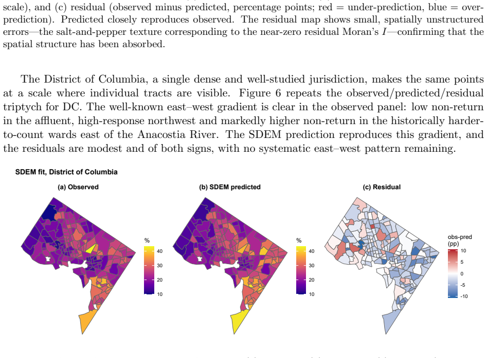
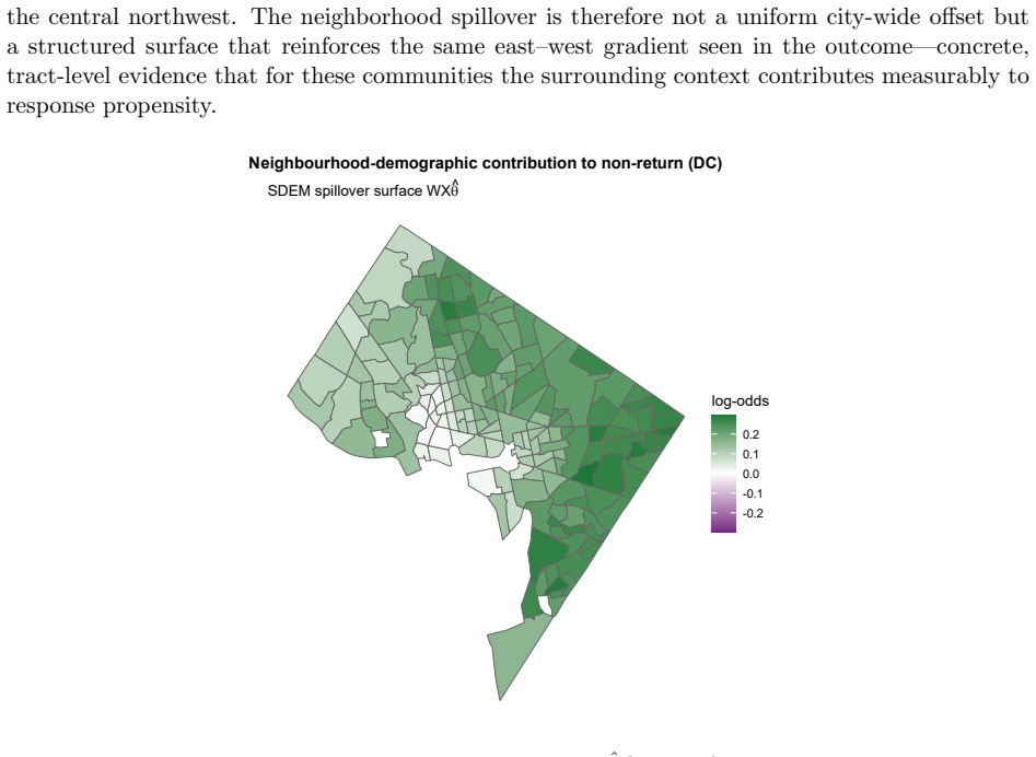
Spatial Dependence in the Self-Response: Spatial Dependence, Modeling, and Operational Consequences
Pith reviewed 2026-07-01 01:29 UTC · model grok-4.3
The pith
Error-type spatial models capture residual dependence in census non-response better than lag processes when tested out of sample.
A machine-rendered reading of the paper's core claim, the machinery that carries it, and where it could break.
Core claim
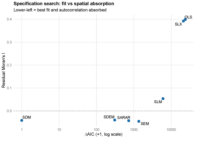
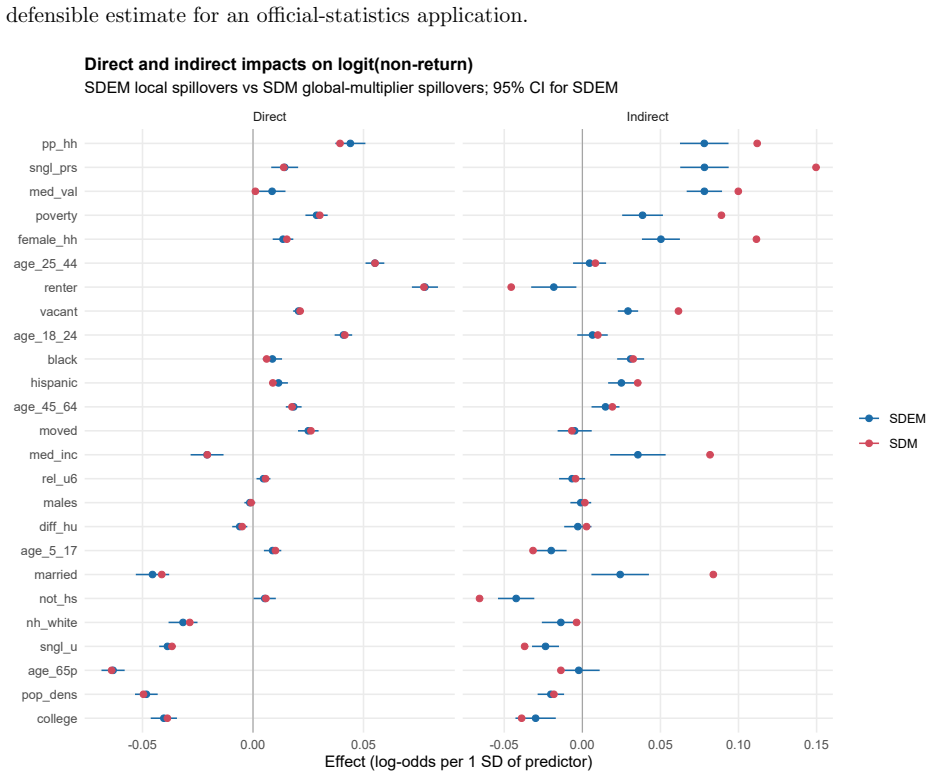
With 71,076 tracts and the twenty-five Erdman-Bates predictors under queen-contiguity weights, OLS produces a Moran's I of 0.399. Formal diagnostics attribute the leftover dependence to error processes. The spatial Durbin model minimizes AIC, yet spatial error models (SEM and SDEM) achieve the best performance under spatial-block validation, while the SDM performs worst out of sample. The SDEM supplies an interpretable middle ground by treating neighborhood effects as local spillovers.
What carries the argument
Comparison of the spatial autoregressive model family (OLS, SAR, SEM, SDM, SDEM) under queen-contiguity weights, ranked by in-sample AIC and by random versus spatial-block cross-validation.
If this is right
- Low Response Score models should incorporate spatial error terms rather than lag terms to improve generalization.
- Local neighborhood demographic effects can be represented as spillovers without requiring a global response-contagion process.
- Official planning instruments of this type should be assessed with spatial-block validation in addition to in-sample fit measures.
- The SDEM specification supplies both statistical performance and direct interpretation of neighboring tract influences.
Where Pith is reading between the lines
- Similar spatial error specifications may improve other geographically clustered survey planning scores that currently rely on plain OLS.
- If tract boundaries or weights definitions change, the relative performance of error versus lag models could shift and should be rechecked.
- The finding that in-sample AIC and spatial validation disagree suggests that many spatial applications would benefit from explicit out-of-sample spatial testing.
Load-bearing premise
Queen-contiguity weights defined on 2010 tract boundaries capture the relevant spatial dependence and the chosen predictors plus spatial terms account for all systematic variation in non-response rates.
What would settle it
Finding that the spatial Durbin model outperforms the spatial error models under repeated spatial-block validation on held-out tracts would falsify the claim that error-type dependence is primary.
Figures


read the original abstract
The U.S.\ Census Bureau's Low Response Score (LRS) is a central planning instrument for identifying places likely to require additional self-response outreach and nonresponse follow-up. The published LRS is intentionally interpretable: it is built from tract-level covariates using an ordinary least squares specification. That transparency, however, leaves open an important question for official statistics: how much spatial structure remains after the own-tract covariates have done their work, and what form does that structure take? Using the observed 2010 Census mail non-return rate for 71,076 U.S. census tracts and the twenty-five Erdman--Bates LRS predictors, this paper compares the full spatial autoregressive model family under queen-contiguity weights and validates the leading candidates with both random and spatial-block cross-validation. OLS leaves strong residual spatial autocorrelation ($I=0.399$). Formal diagnostics and model comparisons indicate that the remaining dependence is primarily error-type rather than a global endogenous lag process. Although the spatial Durbin model minimizes in-sample AIC, spatial-block validation reverses that ranking: the error-family models (SEM/SDEM) generalize best, while the AIC-best SDM is weakest out of sample. The SDEM provides an interpretable middle ground, absorbing residual spatial dependence while representing neighborhood demographic effects as local spillovers. Robustness checks show that these conclusions are invariant to the weights definition and are not an artifact of tract-size-driven heteroskedasticity. The results suggest that LRS-style response models should be evaluated with spatial validation, not only in-sample fit, and that local neighborhood context can be operationally meaningful without invoking a global response-contagion mechanism.
Editorial analysis
A structured set of objections, weighed in public.
Referee Report
Summary. The paper analyzes residual spatial dependence in 2010 U.S. Census tract mail non-response rates (71,076 tracts) after OLS regression on the 25 Erdman-Bates LRS predictors. It reports strong residual Moran's I (0.399), uses LM diagnostics and the full spatial autoregressive family (SAR, SEM, SDM, SDEM, etc.) under queen-contiguity weights, and finds that spatial-block cross-validation reverses the in-sample AIC ranking: error-family models (SEM/SDEM) generalize best while the AIC-best SDM performs worst out-of-sample. The SDEM is presented as an interpretable compromise capturing local spillovers without global lag contagion. Robustness to alternative weights and heteroskedasticity is claimed.
Significance. If the central claim holds, the work is significant for official statistics practice: it shows that reliance on in-sample AIC alone can select models that fail spatial generalization, and that neighborhood demographic spillovers can be modeled operationally via error or Durbin-error specifications without invoking a global endogenous response process. The explicit use of spatial-block CV and the contrast between in-sample and out-of-sample rankings provide a concrete, falsifiable demonstration that is directly relevant to census planning tools such as the Low Response Score.
major comments (2)
- [Abstract] Abstract (robustness paragraph): the claim that 'these conclusions are invariant to the weights definition' is load-bearing for the error-type vs. lag-type classification, yet the abstract provides no enumeration of the alternative weight matrices examined nor any table or figure showing how the LM test statistics or the SEM/SDEM vs. SDM ranking change under those alternatives. Without this, it is impossible to assess whether queen contiguity is merely one convenient choice or whether the lag-vs-error distinction is robust to plausible changes in neighborhood definition.
- [Abstract] Abstract (model comparison and CV paragraph): the reversal of ranking under spatial-block CV is the key empirical result supporting the error-type conclusion, but the abstract does not report the number of blocks, the block-construction rule, or the precise out-of-sample metric (e.g., RMSE, MAE, or log-score) used to declare SEM/SDEM superior. These details are necessary to evaluate whether the spatial-block design truly isolates the dependence structure or inadvertently favors error models by construction.
minor comments (1)
- [Abstract] The abstract states OLS leaves I=0.399 but does not indicate whether this is the raw or residual Moran's I, nor the exact p-value or permutation test used.
Simulated Author's Rebuttal
We thank the referee for these focused comments on the abstract. Both points correctly identify places where additional detail would strengthen the presentation of our robustness and validation results. We address each below and will revise the abstract accordingly.
read point-by-point responses
-
Referee: [Abstract] Abstract (robustness paragraph): the claim that 'these conclusions are invariant to the weights definition' is load-bearing for the error-type vs. lag-type classification, yet the abstract provides no enumeration of the alternative weight matrices examined nor any table or figure showing how the LM test statistics or the SEM/SDEM vs. SDM ranking change under those alternatives. Without this, it is impossible to assess whether queen contiguity is merely one convenient choice or whether the lag-vs-error distinction is robust to plausible changes in neighborhood definition.
Authors: We agree the abstract should be more explicit. The manuscript already reports results under queen contiguity as the primary specification and states that conclusions are invariant under alternatives. To make this transparent in the abstract we will add a parenthetical enumeration of the matrices tested (rook contiguity, k=4 and k=8 nearest-neighbor, and 5 km / 10 km distance-band weights) and note that both the LM diagnostics and the out-of-sample ranking of error-family versus lag-family models remain unchanged. A concise supplementary table summarizing the key LM statistics and CV rankings across weights will also be referenced. revision: yes
-
Referee: [Abstract] Abstract (model comparison and CV paragraph): the reversal of ranking under spatial-block CV is the key empirical result supporting the error-type conclusion, but the abstract does not report the number of blocks, the block-construction rule, or the precise out-of-sample metric (e.g., RMSE, MAE, or log-score) used to declare SEM/SDEM superior. These details are necessary to evaluate whether the spatial-block design truly isolates the dependence structure or inadvertently favors error models by construction.
Authors: The referee is correct that these operational details belong in the abstract. The spatial-block CV used 100 blocks formed by k-means clustering on tract centroids (ensuring no shared borders between training and test blocks), with RMSE as the out-of-sample metric. We will revise the abstract sentence to read: 'spatial-block cross-validation (100 k-means centroid blocks, RMSE) reverses that ranking: the error-family models (SEM/SDEM) generalize best...' This addition directly addresses the concern without lengthening the abstract beyond its limit. revision: yes
Circularity Check
No significant circularity; claims rest on held-out validation
full rationale
The paper's core result—that residual dependence after the 25 Erdman-Bates covariates is primarily error-type (SEM/SDEM) rather than lag-type (SDM/SAR), and that spatial-block CV reverses the AIC ranking—is obtained by fitting standard spatial autoregressive models to the 2010 tract data under queen-contiguity weights and then evaluating predictive performance on spatially blocked hold-out sets. No equation reduces a fitted quantity to itself by construction, no parameter is estimated on a subset and then relabeled a prediction, and no uniqueness theorem or prior self-citation is invoked to force the model family. The derivation therefore remains self-contained against external benchmarks (the observed non-response rates and the explicit cross-validation partitions).
Axiom & Free-Parameter Ledger
free parameters (1)
- spatial autoregressive coefficient(s)
axioms (1)
- domain assumption Queen-contiguity weights matrix correctly encodes spatial neighbors for census tracts
Reference graph
Works this paper leans on
-
[1]
K., Florax, R., and Yoon, M
Anselin, L., Bera, A. K., Florax, R., and Yoon, M. J. (1996). Simple diagnostic tests for spatial dependence. Regional Science and Urban Economics, 26(1), 77--104
1996
-
[2]
Burridge, P. (1981). Testing for a common factor in a spatial autoregression model. Environment and Planning A, 13(7), 795--800
1981
-
[3]
Census Bureau
U.S. Census Bureau. (2026). Updating the Planning Database with the latest socioeconomic, demographic and housing data. Random Samplings Blog. https://www.census.gov/newsroom/blogs/random-samplings/2026/03/updating-the-planning-database.html
2026
-
[4]
Elhorst, J. P. (2010). Applied spatial econometrics: raising the bar. Spatial Economic Analysis, 5(1), 9--28
2010
-
[5]
Erdman, C., and Bates, N. (2017). The Low Response Score (LRS): A metric to locate, predict, and manage hard-to-survey populations. Public Opinion Quarterly, 81(1), 144--156
2017
-
[6]
Goulard, M., Laurent, T., and Thomas-Agnan, C. (2017). About predictions in spatial autoregressive models: optimal and almost optimal strategies. Spatial Economic Analysis, 12(2--3), 304--325
2017
-
[7]
H., and Prucha, I
Kelejian, H. H., and Prucha, I. R. (2010). Specification and estimation of spatial autoregressive models with autoregressive and heteroskedastic disturbances. Journal of Econometrics, 157(1), 53--67
2010
-
[8]
LeSage, J., and Pace, R. K. (2009). Introduction to Spatial Econometrics. Chapman and Hall/CRC, Boca Raton
2009
-
[9]
K., and LeSage, J
Pace, R. K., and LeSage, J. P. (2008). A spatial Hausman test. Economics Letters, 101(3), 282--284
2008
-
[10]
R., et al
Roberts, D. R., et al. (2017). Cross-validation strategies for data with temporal, spatial, hierarchical, or phylogenetic structure. Ecography, 40(8), 913--929
2017
discussion (0)
Sign in with ORCID, Apple, or X to comment. Anyone can read and Pith papers without signing in.