pith. sign in

arxiv: 2606.08823 · v1 · pith:LQOULCEUnew · submitted 2026-06-07 · 🌊 nlin.SI

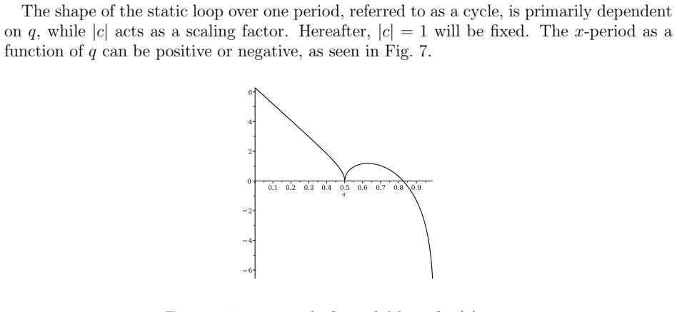
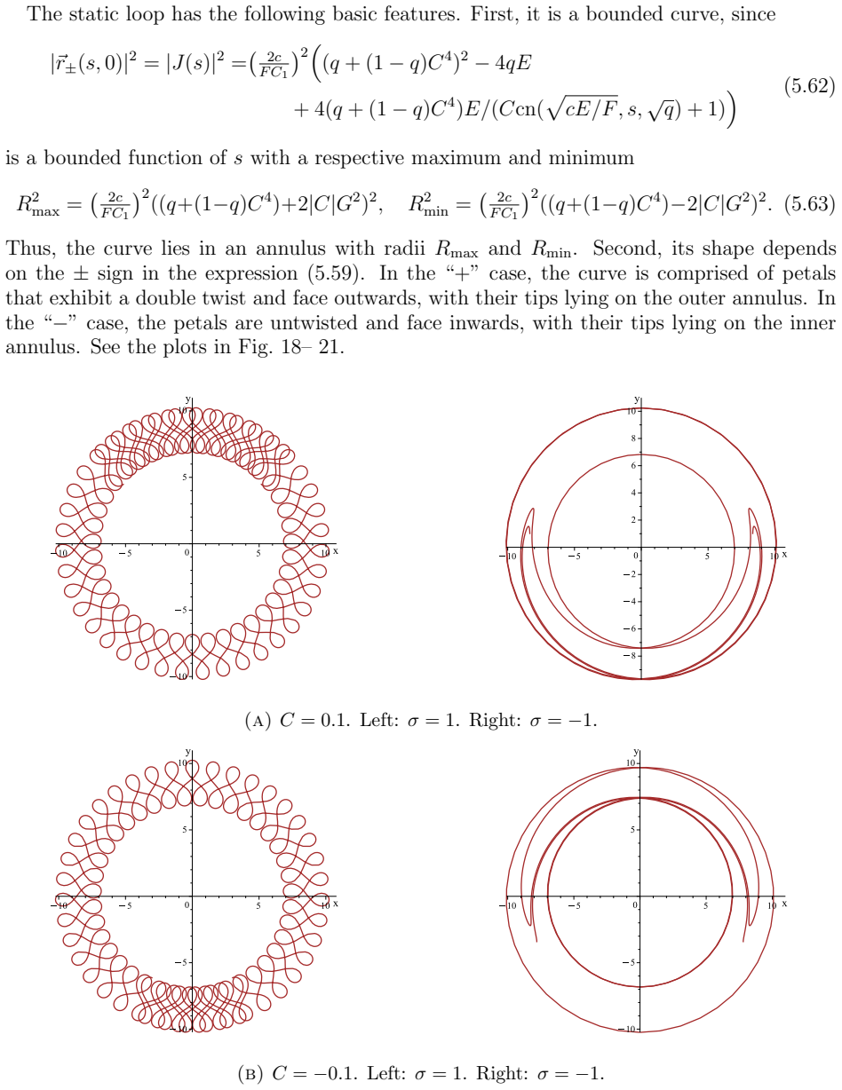
Geometric curve flows in the plane and mKdV loop solutions

Pith reviewed 2026-06-27 17:12 UTC · model grok-4.3

classification 🌊 nlin.SI
keywords geometric curve flowsmodified Korteweg-de Vries equationtravelling wavesloop solutionssolitonscnoidal wavesquadrature formulaclosed curves
0
0 comments X

The pith

mKdV travelling waves yield explicit geometric curve flows in the plane that form either travelling loops or rotating loops via a quadrature formula.

A machine-rendered reading of the paper's core claim, the machinery that carries it, and where it could break.

The paper takes the established link between plane curve evolution and the mKdV equation and applies it to every class of mKdV travelling wave. A single integral formula converts each wave into the curve's tangent angle as a function of arc length, producing concrete shapes. These shapes separate into two families: loops that translate without rotating, generated by solitons and periodic cnoidal or dnoidal waves, and loops that rotate while moving, generated by waves on a background or by rational solutions. The work then determines the parameter values that make any of these loops close on themselves.

Core claim

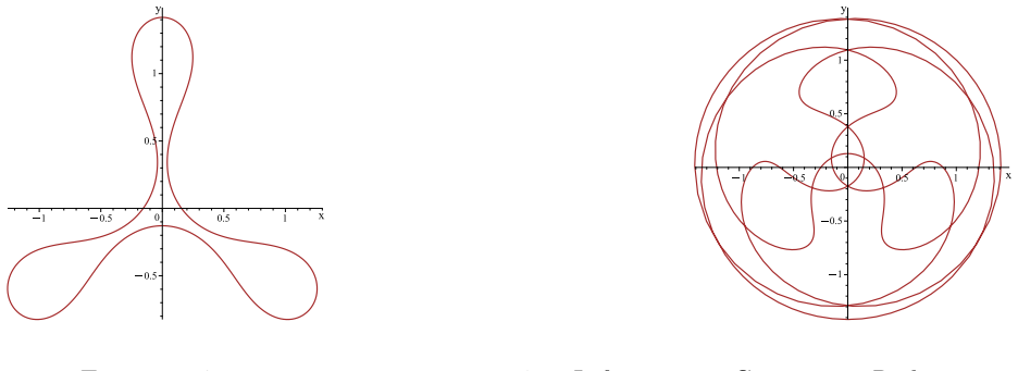
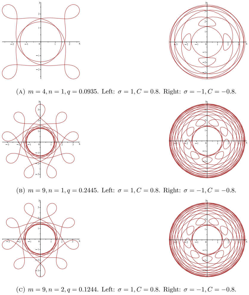
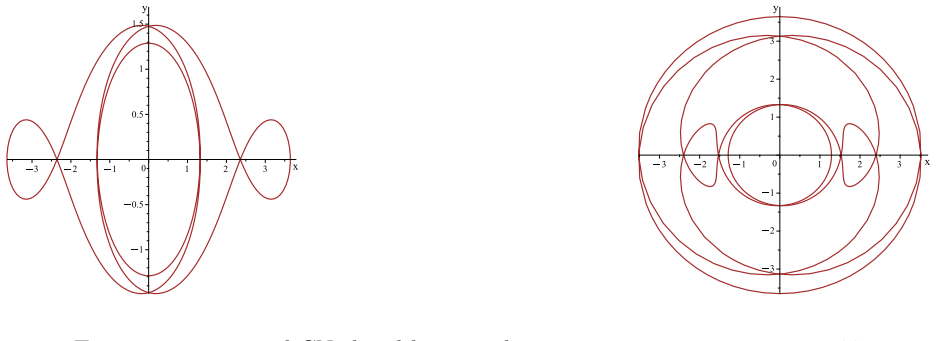
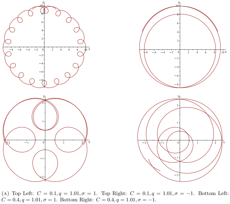
For every type of mKdV travelling wave the corresponding plane curve flow is obtained by quadrature from the wave profile; the resulting curves fall into travelling loops (from solitons, cnoidal waves, and dnoidal waves) and rotating loops (from solitary waves on nonzero background, rational waves, and rational elliptic waves), with explicit conditions for closure of both open and closed periodic loops, including a rational-cosine specialization.

What carries the argument

The quadrature formula that integrates the mKdV travelling-wave profile to obtain the curve's tangent angle as a function of arc length.

If this is right

  • Soliton, cnoidal, and dnoidal mKdV waves produce translating loop curves whose shape is fixed by a single integral.
  • Background and rational mKdV waves produce rotating loops whose angular speed is set by the background value.
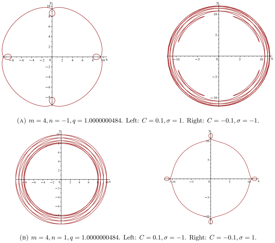
  • Rational elliptic mKdV waves produce periodic rotating loops, some of which close after a finite number of turns.
  • A further reduction of the periodic case yields rational cosine loops whose curvature is a rational function of cosine.
  • Closed loops exist only when the integrated phase advance over one period is an integer multiple of 2π.

Where Pith is reading between the lines

These are editorial extensions of the paper, not claims the author makes directly.

  • The quadrature method supplies a direct geometric picture of every mKdV travelling wave as an actual plane curve, which could be used to test numerical integrators of the curve flow.
  • Because the same quadrature works for both open and closed loops, it may extend to other integrable curve flows whose curvature satisfies related nonlinear equations.
  • The distinction between translating and rotating families suggests a conserved quantity (total turning or enclosed area) that separates the two classes.

Load-bearing premise

The standard correspondence between mKdV solutions and geometric curve flows in the plane continues to hold exactly for the travelling-wave profiles examined here.

What would settle it

Compute one explicit curve from the quadrature formula applied to a known mKdV soliton and check whether its time evolution satisfies the mKdV-derived curvature flow equation at more than one point along the curve.

Figures

Figures reproduced from arXiv: 2606.08823 by Jaskaran Maan, Stephen C. Anco.

Figure 1
Figure 1. Figure 1: Phase plane for ∆ > 0. c = 3/2, C1 = 1/2 Case ∆ > 0: In this case, c > 0 must hold and then the cubic U 3 − 2cU + 2C1 = (U − U∗1)(U − U∗2)(U − U∗3) = 0 has three distinct real roots, which can be ordered U∗1 < U∗2 < U∗3. The first integral (2.6) comprises three family of closed curves. There is one family around each of the points (U∗1, 0) and (U∗3, 0). A double homoclinic orbit through (U∗2, 0) separates … view at source ↗
Figure 2
Figure 2. Figure 2: Phase plane for ∆ < 0. (Left) c = −3/2, C1 = 3/2 (Right) c = 3/2, C1 = 2 [PITH_FULL_IMAGE:figures/full_fig_p005_2.png] view at source ↗
Figure 3
Figure 3. Figure 3: Phase plane for ∆ = 0. c = 3/2, C1 = 1 the separable ODE (2.4): ± Z K(ξ) K0 dK q 1 4K4 − cK2 − 2C1K − 2C2 = ξ − ξ0 (2.8) where K0 is the minimum or maximum of the solution, as given by K(ξ0) = K0 and K′ (ξ0) = 0. Evaluation of the quadrature leads to the following result. 5 [PITH_FULL_IMAGE:figures/full_fig_p005_3.png] view at source ↗
Figure 4
Figure 4. Figure 4: mKdV soliton loop, c = 1. The loop (5.6) is open, has a single peak at s = 0, and asymptotically approaches a straight line as |s| → ∞. Note that s = ∞ corresponds to (−∞, 0) and s = −∞ corresponds 20 [PITH_FULL_IMAGE:figures/full_fig_p020_4.png] view at source ↗
Figure 5
Figure 5. Figure 5: mKdV rational loop The static loop has the following features. It asymptotically winds around a circle of radius 1/|b| as |s| → ∞, as shown by |⃗r(s, 0)| = 1 |b| r b 2s 2 + 9 b 2s 2 + 1 = 1 |b| + O(1/s2 ), ϑs = K(s) = b + O(1/s2 ). (5.16) This winding is counter-clockwise for b > 0, and clockwise for b < 0. The loop has a single twist that forms a smaller self-intersecting loop whose peak is at s = 0. Its … view at source ↗
Figure 6
Figure 6. Figure 6: The static loop has the following features, which are similar to those of the rational loop (5.28). It asymptotically winds around a circle of radius 1/|b| as |s| → ∞, as shown by |⃗r±(s, 0)| = 1 |b|B2 q K′ (s) 2 + ( 1 2K(s) 2 − c) 2 = 1 |b| + O(1/s2 ), ϑs = K(s) = b + O(1/s2 ) (5.29) where the winding is counter-clockwise for b > 0, and clockwise for b < 0. There is a choice of ± sign in the loop expressi… view at source ↗
Figure 6
Figure 6. Figure 6: mKdV soliton on a non-zero background, c = 1. such that xs(|s|, 0) = cos(ϑ(|s|)) = 0. This determines s = ζ/b where ζ is the smallest positive root of the equation ±sgn(b) √ a 2 + 1 − 1 a tanh( 1 2 aζ) = tan( 1 8 (π − 2ζ)), a = F/|b| = q (c/b2 ) − 3 2 > 0. (5.31) Substituting s = ζ/b into |x(s, 0)−x(−s, 0)| = 2|x(s)| given by the x-component of expression (5.28) then yields w = 2c − K(ζ/b) 2 |b|(c − 1 2 b … view at source ↗
Figure 7
Figure 7. Figure 7: x-period of cnoidal loop for |c| = 1. For q < 1 2 , the cycle is an untwisted loop that is symmetric under s → −s. It has maximum amplitude 4p F1/c, while its minimum amplitude is 0. In addition, its speed is negative. See [PITH_FULL_IMAGE:figures/full_fig_p027_7.png] view at source ↗
Figure 11
Figure 11. Figure 11: The two halves of the loop will exactly overlap such that a closed loop is formed when x(s, 0) returns to the same value after one period (5.42), namely x(0, 0) = x(4K(p cq/(2q − 1)), 0) so that the x-periodic is zero. This condition yields q = qclosed ≃ 0.8261. The resulting closed loop has the shape of a figure 8 with height ≃ 2.936 and width ≃ 0.546, respectively. See [PITH_FULL_IMAGE:figures/full_fig… view at source ↗
Figure 13
Figure 13. Figure 13: The last touch occurs for q = q ∗ 1 ≃ 0.886. See [PITH_FULL_IMAGE:figures/full_fig_p027_13.png] view at source ↗
Figure 8
Figure 8. Figure 8: cnoidal loop, c = −1 [PITH_FULL_IMAGE:figures/full_fig_p028_8.png] view at source ↗
Figure 9
Figure 9. Figure 9: cnoidal loop, c = 1, q = 0.65. 5.5. dnoidal loops. Dnoidal mKdV waves (2.16) are bright/dark corresponding to the ± sign. Similarly to the cnoidal solutions, these waves (2.16) yield loop solutions obtained by evaluation of the parametric integrals (4.3) and (4.1b) together with expression (4.2b), where 28 [PITH_FULL_IMAGE:figures/full_fig_p028_9.png] view at source ↗
Figure 10
Figure 10. Figure 10: cnoidal loop, c = 1, q = q∗1 ≃ 0.7317 [PITH_FULL_IMAGE:figures/full_fig_p029_10.png] view at source ↗
Figure 11
Figure 11. Figure 11: cnoidal loop, c = 1. Left: q ≃ 0.799. Right: q ≃ 0.811 [PITH_FULL_IMAGE:figures/full_fig_p029_11.png] view at source ↗
Figure 12
Figure 12. Figure 12: closed cnoidal loop: q = qclosed ≃ 0.8261, c = 1. C = 0. Note that q and c obey the inequality q > 1, c > 0. (5.45) 29 [PITH_FULL_IMAGE:figures/full_fig_p029_12.png] view at source ↗
Figure 13
Figure 13. Figure 13: cnoidal loop, c = 1. Left: q ≃ 0.849. Right: q ≃ 0.859 [PITH_FULL_IMAGE:figures/full_fig_p030_13.png] view at source ↗
Figure 14
Figure 14. Figure 14: cnoidal loop q = q ∗ 1 ≃ 0.886, c = 1. The first parametric integral yields ϑ = ±2 arctan  sn(q p c/F1 s, 1/ √q) cn(q p c/F1 s, 1/ √q)  = ±2 am(q p c/F1 s, 1/ √ q) (5.46) where am denotes the Jacobi amplitude function. This gives e iϑ(s) = ∓sn(q p c/F1 s, 1/ √q) + icn(q p c/F1 s, 1/ √q) ±sn(q p c/F1 s, 1/ √q) + icn(q p c/F1 s, 1/ √q) . (5.47) Then the second parametric integral gives Z s 0 e iϑ(s) ds = … view at source ↗
Figure 15
Figure 15. Figure 15: cnoidal loop, c = 1, q ≃ 0.999. Substitution into the loop equation (4.1b) produces z(s, t) = 1 2q−1 ct − (2q − 1)s + 2p F1/c E [PITH_FULL_IMAGE:figures/full_fig_p031_15.png] view at source ↗
Figure 16
Figure 16. Figure 16: x-period of dnoidal loop for c = 1. (a) Left: q = 1.01. Right: q = 1.1. (b) Left: q = 1.5. Right: q = 2.5 [PITH_FULL_IMAGE:figures/full_fig_p032_16.png] view at source ↗
Figure 17
Figure 17. Figure 17: dnoidal loop, c = 1. and winding rate W = 4 π r cq 2q − 1 E(1/ √ q). (5.54) 32 [PITH_FULL_IMAGE:figures/full_fig_p032_17.png] view at source ↗
Figure 18
Figure 18. Figure 18: rational CN open loops with c = 1, q = 0.9. 34 [PITH_FULL_IMAGE:figures/full_fig_p034_18.png] view at source ↗
Figure 19
Figure 19. Figure 19: rational CN open loops with c = 1, q = 0.2. 35 [PITH_FULL_IMAGE:figures/full_fig_p035_19.png] view at source ↗
Figure 20
Figure 20. Figure 20: rational CN open loops with c = 1, q = 0.9. 36 [PITH_FULL_IMAGE:figures/full_fig_p036_20.png] view at source ↗
Figure 21
Figure 21. Figure 21: rational CN open loops with c = 1, q = 0.4. From the results in [PITH_FULL_IMAGE:figures/full_fig_p037_21.png] view at source ↗
Figure 22
Figure 22. Figure 22: Largest and smallest ratio for n/m in the case σsgn(C) = 1. 38 [PITH_FULL_IMAGE:figures/full_fig_p038_22.png] view at source ↗
Figure 23
Figure 23. Figure 23: rational CN closed loops with c = 1. 39 [PITH_FULL_IMAGE:figures/full_fig_p039_23.png] view at source ↗
Figure 24
Figure 24. Figure 24: m = 3, n = 1, q = 0.3549. Left: σ = 1, C = 0.35. Right: σ = −1, C = −0.35. 40 [PITH_FULL_IMAGE:figures/full_fig_p040_24.png] view at source ↗
Figure 25
Figure 25. Figure 25: rational CN closed loops with c = 1. 41 [PITH_FULL_IMAGE:figures/full_fig_p041_25.png] view at source ↗
Figure 26
Figure 26. Figure 26: rational CN closed loops with c = 1. 42 [PITH_FULL_IMAGE:figures/full_fig_p042_26.png] view at source ↗
Figure 27
Figure 27. Figure 27: rational CN closed loops with c = 1. 43 [PITH_FULL_IMAGE:figures/full_fig_p043_27.png] view at source ↗
Figure 28
Figure 28. Figure 28: rational CN closed loops with c = 1, m = 2, n = −1. 44 [PITH_FULL_IMAGE:figures/full_fig_p044_28.png] view at source ↗
Figure 29
Figure 29. Figure 29: rational CN closed loops with c = 1, m = 2, n = −1, q = 0.2244. Left: σ = 1, C = 0.9. Right: σ = −1, C = −0.9. 5.7. Rational dn loops. Periodic rational-dn mKdV waves with q > 1 are bright/dark corresponding to the ± sign in expression (2.15). The resulting loop solutions are obtained similarly to the rational cn loops by evaluation of the parametric integral (4.3) and the algebraic formula (4.1a), in add… view at source ↗
Figure 30
Figure 30. Figure 30: rational DN open loops c = 1 47 [PITH_FULL_IMAGE:figures/full_fig_p047_30.png] view at source ↗
Figure 31
Figure 31. Figure 31: rational DN open loops c = 1. 48 [PITH_FULL_IMAGE:figures/full_fig_p048_31.png] view at source ↗
Figure 32
Figure 32. Figure 32: rational DN open loops C = 0.9, q = 1.2, c = 1. Left: σ = 1. Right:σ = −1. These curves have complicated expressions for the winding number (4.24) and the mean￾winding rate (4.1), which arise from the results in [PITH_FULL_IMAGE:figures/full_fig_p049_32.png] view at source ↗
Figure 33
Figure 33. Figure 33: rational DN closed loops c = 1. 50 [PITH_FULL_IMAGE:figures/full_fig_p050_33.png] view at source ↗
Figure 34
Figure 34. Figure 34: rational DN closed loops c = 1 51 [PITH_FULL_IMAGE:figures/full_fig_p051_34.png] view at source ↗
Figure 35
Figure 35. Figure 35: rational DN closed loops c = 1 5.8. Rational cosine loops. For the rational-cosine mKdV waves (2.13), the corresponding loop solutions are derived by specializing the rational cn loops to the case q = 0. Note that c and C obey the inequalities c > 0 and 0 < C2 < 1. It will be convenient now to let F = (1 − C)/(1 + C), G = (1 − C 2 )/(1 + 2C 2 ). (5.79) The parametric integral (4.3) is given by ϑ(s) = ± p… view at source ↗
Figure 36
Figure 36. Figure 36: rational cosine open loops c = 1. 53 [PITH_FULL_IMAGE:figures/full_fig_p053_36.png] view at source ↗
Figure 37
Figure 37. Figure 37: rational cosine closed loops c = 1 54 [PITH_FULL_IMAGE:figures/full_fig_p054_37.png] view at source ↗
Figure 38
Figure 38. Figure 38: rational cosine closed loops c = 1 6. Concluding remarks The present work has derived the loop solutions corresponding to each type of mKdV travelling wave. These loop solutions can be cleanly divided into two broad types: travelling loops, and rotating loops. Travelling loops arise from mKdV solitons and cnoidal (Jacobi cn) waves, the latter being periodic. Rotating loops can be subdivided into asymptoti… view at source ↗
Figure 39
Figure 39. Figure 39: rational cosine closed loops c = 1 For future work, the loop solutions corresponding to other (non-travelling wave) mKdV solutions can be pursued. Specifically, breathers and multi-solitons — both on a zero back￾ground or a non-zero background — can be expected to produce interacting dynamical loops with interesting properties. Appendix A. Appendix: Ellipitic function identities All of the relevant algebr… view at source ↗
read the original abstract

There is a well known correspondence between geometric curve flows in the Euclidean plane and solutions of the modified Korteweg-de Vries (mKdV) equation. For each type of mKdV travelling wave, the resulting geometric curve flows are derived here through a simple quadrature formula and studied in detail. These curve flows can be divided into two broad types: travelling loops, and rotating loops. Travelling loops are shown to arise from mKdV solitons, cnoidal (Jacobi cn) and dnoidal (Jacobi dn) waves, the latter being periodic. Rotating loops comprise asymptotically circular ones that are obtained from both mKdV solitary waves on a non-zero background and mKdV rational waves, as well as periodic ones that are produced by mKdV rational elliptic (cn and dn) waves. A specialization of periodic loops, both open and closed, is shown to yield rational cosine loops. An explicit description of each of these types of curve flows is used to characterize their main features, including the condition under which closed loops exist.

Editorial analysis

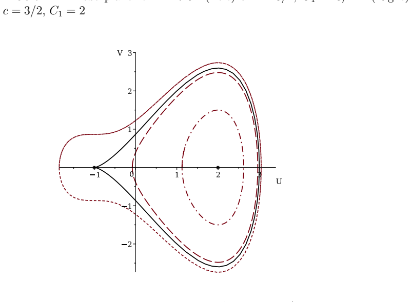
A structured set of objections, weighed in public.

Desk editor's note, referee report, simulated authors' rebuttal, and a circularity audit. Tearing a paper down is the easy half of reading it; the pith above is the substance, this is the friction.

Referee Report

0 major / 2 minor

Summary. The manuscript studies the geometric curve flows in the Euclidean plane that arise from travelling-wave solutions of the mKdV equation under the standard curvature-flow correspondence. For solitons, cnoidal (Jacobi cn), dnoidal (Jacobi dn), rational, and rational-elliptic waves, the flows are obtained explicitly by quadrature; the resulting motions are classified into travelling loops (from zero-background solitons and periodic waves) and rotating loops (from nonzero-background solitary waves, rational waves, and periodic rational-elliptic waves), with a further specialization to rational cosine loops. Closed-loop existence conditions are derived from the explicit integrals.

Significance. The explicit quadrature derivations supply concrete, parameter-free geometric realizations of standard mKdV travelling waves as loop evolutions. This classification into travelling versus rotating loops, together with the closed-loop criteria, furnishes a useful dictionary between integrable PDE solutions and planar curve dynamics that can be checked directly against the integrals.

minor comments (2)
  1. [Abstract] Abstract: the phrase 'rational elliptic (cn and dn) waves' is used without a preceding definition or citation; a brief parenthetical reminder of the form of these solutions would aid readers unfamiliar with the rational-elliptic mKdV family.
  2. The manuscript would benefit from a short table or enumerated list summarizing the quadrature formula, the resulting loop type, and the closed-loop condition for each wave family.

Simulated Author's Rebuttal

0 responses · 0 unresolved

We thank the referee for their positive assessment of the manuscript and for recommending acceptance with no major comments.

Circularity Check

0 steps flagged

No significant circularity

full rationale

The derivation begins from the standard, externally established correspondence between Euclidean plane curve flows and mKdV solutions, then integrates the resulting curvature ODEs by quadrature for known travelling-wave profiles. All subsequent classification into travelling/rotating loops and closed-loop conditions follows directly from the explicit integrals without any parameter fitting, self-referential definitions, or load-bearing self-citations. The central steps remain independent of the paper's own outputs.

Axiom & Free-Parameter Ledger

0 free parameters · 0 axioms · 0 invented entities

Abstract only; no explicit free parameters, axioms, or invented entities described.

pith-pipeline@v0.9.1-grok · 5713 in / 967 out tokens · 15951 ms · 2026-06-27T17:12:03.162876+00:00 · methodology

discussion (0)

Sign in with ORCID, Apple, or X to comment. Anyone can read and Pith papers without signing in.

Forward citations

Cited by 1 Pith paper

Reviewed papers in the Pith corpus that reference this work. Sorted by Pith novelty score.

  1. Perturbation theory for kinks of the defocusing modified Korteweg-de Vries equation

    nlin.SI 2026-06 unverdicted novelty 6.0

    Develops integrable perturbation theory for defocusing mKdV kinks, derives completeness and adjoint relations, obtains leading-order evolution equations for kink parameters, and shows generic radiative shelf formation...

Reference graph

Works this paper leans on

19 extracted references · cited by 1 Pith paper

  1. [1]

    Nakayama, H

    K. Nakayama, H. Segur, M. Wadati, Integrability and the motion of curves, Phys. Rev. Lett. 69 (1992), 2603–2606

  2. [2]

    Goldstein and D.M

    R.E. Goldstein and D.M. Petrich, Solitons, Euler’s equation, and the geometry of curve motion. In Singularities in Fluids, Plasmas and Optics, 93–109, Eds. R.E. Caflisch, G.G. Papanicolaou, Kluwer 1993

  3. [3]

    Goldstein and D.M

    R.E. Goldstein and D.M. Petrich, The Korteweg–de Vries hierarchy as dynamics of closed curves in the plane, Phys. Rev. Lett. 67(23) (1991), 3203–3206

  4. [4]

    Goldstein and D.M

    R.E. Goldstein and D.M. Petrich, Solitons, Euler’s equation, and vortex patch dynamics, Phys. Rev. Lett. 69 (1992), 555–558

  5. [5]

    Wexler, A.T

    C. Wexler, A.T. Dorsey, Solitons on the edge of a two-dimensional electron system, Phys. Rev. Lett. 82(3) (1999), 620–623

  6. [6]

    Wexler, A.T

    C. Wexler, A.T. Dorsey, Contour dynamics, waves, and solitons in the quantum Hall effect, Phys. Rev. B 60(15) (1999), 10971–10983

  7. [7]

    Vassilev, P.A

    V.M. Vassilev, P.A. Djondjorov, I.M. Mladenov, Cylindrical equilibrium shapes of fluid membranes, J. Phys. A: Math. Theor. 41 (2008), 435201

  8. [8]

    Nishinari, Nonlinear dynamics of solitary waves in an extensible rod, Proc

    K. Nishinari, Nonlinear dynamics of solitary waves in an extensible rod, Proc. Roy. Soc. A 453 (1997), 817–833

  9. [9]

    Nakayama, M

    K. Nakayama, M. Wadati, Motion of curves in the plane, J. Phys. Soc. Jpn. 62(2) (1993), 473–479

  10. [10]

    Anco, H-R

    S.C. Anco, H-R. Nayeri, E. Recio, Travelling wave solutions on a non-zero background for the gener- alized Korteweg–de Vries equation, J. Phys. A: Math. Theor. 54 (2021) 085701. 58

  11. [11]

    Miura, C.S

    R.M. Miura, C.S. Gardner, M.D. Kruskal, Kortewegde Vries Equation and Generalizations. II. Exis- tence of Conservation Laws and Constants of Motion, J. Math. Phys. 9 (1968), 1204–1209

  12. [12]

    Anco, Conservation laws of scaling-invariant field equations, J

    S.C. Anco, Conservation laws of scaling-invariant field equations, J. Phys. A: Math. Gen. 36 (2003), 8623–8638

  13. [13]

    Guggenheimer,Differential Geometry, McGraw-Hill, 1963

    H. Guggenheimer,Differential Geometry, McGraw-Hill, 1963

  14. [14]

    Anco, Group-invariant soliton equations and bi-Hamiltonian geometric curve flows in Riemannian symmetric spaces, J

    S.C. Anco, Group-invariant soliton equations and bi-Hamiltonian geometric curve flows in Riemannian symmetric spaces, J. Geom. Phys. 58 (2008), 1–37

  15. [15]

    Ablowtiz, P.A

    M.A. Ablowtiz, P.A. Clarkson,Solitons, Nonlinear Evolution Equations and Inverse Scattering, Cam- bridge University Press, 2010

  16. [16]

    Olver,Applications of Lie Groups to Differential Equations, Springer-Verlag, New York, 1993

    P.J. Olver,Applications of Lie Groups to Differential Equations, Springer-Verlag, New York, 1993

  17. [17]

    Abramowitz, I

    M. Abramowitz, I. Stegun,Handbook of Mathematical Functions, Applied Mathematics Series 55, National Bureau of Standards, 1964

  18. [18]

    Mari Beffa, J.A

    G. Mari Beffa, J.A. Sanders, J.-P. Wang, Integrable systems in three-dimensional Riemannian geome- try, J. Nonlinear Sci. 12 (2002), 143–167

  19. [19]

    Dorfman,Dirac Structures and Integrability of Nonlinear Evolution Equations, John-Wiley, 1993

    I. Dorfman,Dirac Structures and Integrability of Nonlinear Evolution Equations, John-Wiley, 1993. 59