Estimating the Number of Components in Finite Mixture Models via Variational Approximation

Chenyang Wang; Yun Yang

arxiv: 2404.16746 · v2 · submitted 2024-04-25 · 📊 stat.ME · math.ST· stat.ML· stat.TH

Estimating the Number of Components in Finite Mixture Models via Variational Approximation

Chenyang Wang , Yun Yang This is my paper

Pith reviewed 2026-05-24 02:34 UTC · model grok-4.3

classification 📊 stat.ME math.STstat.MLstat.TH

keywords finite mixture modelsvariational BayesELBOmodel selectionconsistencymean-field approximationcomponent estimation

0 comments

The pith

Maximizing the ELBO from mean-field variational approximation consistently selects the number of components in finite mixture models.

A machine-rendered reading of the paper's core claim, the machinery that carries it, and where it could break.

This paper establishes matching upper and lower bounds on the evidence lower bound for finite mixture models using mean-field variational approximation, without needing conjugate priors. These bounds imply that selecting the model by maximizing the ELBO will consistently recover the true number of components as sample size grows. The proof also shows that the variational approximation automatically eliminates extra components when too many are specified, mirroring the behavior of the true posterior, and yields parameter estimates with a near n to the power of negative one half rate. This approach offers a variational method for model selection in mixtures that is both theoretically justified and computationally feasible.

Core claim

The authors prove that the ELBO has matching upper and lower bounds for finite mixture models, establishing that its maximization leads to consistent estimation of the number of components. The mean-field approximation inherits the singularity-driven stability of the posterior that removes superfluous components under overspecification.

What carries the argument

Matching upper and lower bounds on the ELBO derived from the mean-field variational family, which exploits model singularity to prune extra components.

If this is right

Maximizing the ELBO yields a consistent estimator for the number of mixture components.
The variational posterior eliminates extra components under model overspecification.
Parameter estimates achieve a convergence rate of n to the minus one half up to logarithmic factors under overspecification.
The results hold without assuming conjugate priors on the parameters.

Where Pith is reading between the lines

These are editorial extensions of the paper, not claims the author makes directly.

This suggests potential for similar ELBO-based selection in other models with singular parameter spaces.
Empirical validation could involve testing on high-dimensional mixtures where traditional methods struggle.
Extensions might include deriving explicit constants in the bounds for practical sample size calculations.

Load-bearing premise

The mean-field variational family is assumed flexible enough to capture the stable posterior behavior that eliminates extra components under overspecification.

What would settle it

A simulation study where the number of components selected by maximizing the ELBO differs from the true number for large sample sizes would contradict the consistency result.

Figures

Figures reproduced from arXiv: 2404.16746 by Chenyang Wang, Yun Yang.

**Figure 1.** Figure 1: Plots of (LbK − LbK∗ )/ log n versus K with fixed n. generated from a d-dimensional Gaussian mixture model with K∗ = 2 components and d = 6. We use a common variance-covariance matrix for the mixture components, which is the identity matrix I and treated as known. The true mixing weights are w ∗ 1 = w ∗ 2 = 1/2 and the two true location parameters are η ∗ 1 = −2/ √ d · 1 and η ∗ 2 = 2/ √ d · 1, where 1 den… view at source ↗

**Figure 2.** Figure 2: Plots of LbK − log p(Xn |θ) [PITH_FULL_IMAGE:figures/full_fig_p022_2.png] view at source ↗

**Figure 3.** Figure 3: Plots of (LbK − LbK∗ )/ log n versus ϕ0 with fixed K. the lines for larger ϕ0 = {3.5, 4.5, 6} exceeding the critical threshold (d + 1)/2 = 3.5 remains essentially unchanged across different K. For ϕ0 < 3.5, the lines becomes less steep compared to ϕ = 3.5 as K increases. Those empirical observations again align well with the prediction from our theory. Finally, to examine the stability behavior of the vari… view at source ↗

**Figure 4.** Figure 4: Percentages of selecting the correct model in the multivariate Gaussian mixture [PITH_FULL_IMAGE:figures/full_fig_p026_4.png] view at source ↗

**Figure 5.** Figure 5: ELBO and true evidence values for Gaussian mixture model with K components [PITH_FULL_IMAGE:figures/full_fig_p027_5.png] view at source ↗

read the original abstract

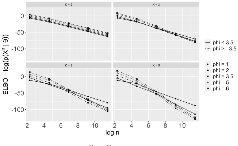
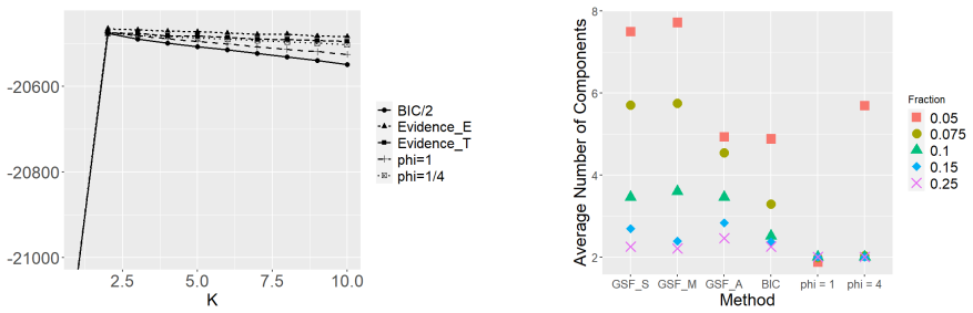
This work introduces a new method for selecting the number of components in finite mixture models (FMMs) using variational Bayes, inspired by the large-sample properties of the Evidence Lower Bound (ELBO) derived from mean-field (MF) variational approximation. Specifically, we establish matching upper and lower bounds for the ELBO without assuming conjugate priors, suggesting the consistency of model selection for FMMs based on maximizing the ELBO. As a by-product of our proof, we demonstrate that the MF approximation inherits the stable behavior (benefited from model singularity) of the posterior distribution, which tends to eliminate the extra components under model misspecification where the number of mixture components is over-specified. This stable behavior also leads to the $n^{-1/2}$ convergence rate for parameter estimation, up to a logarithmic factor, under this model overspecification. Empirical experiments are conducted to validate our theoretical findings and compare with other state-of-the-art methods for selecting the number of components in FMMs.

Editorial analysis

A structured set of objections, weighed in public.

Desk editor's note, referee report, simulated authors' rebuttal, and a circularity audit. Tearing a paper down is the easy half of reading it; the pith above is the substance, this is the friction.

Desk Editor's Note private letter to a colleague

The paper proves matching ELBO bounds for non-conjugate finite mixture models and claims this yields consistent selection of the number of components, plus a side result that mean-field variational posteriors inherit the true posterior's pruning of extra components under overspecification.

read the letter

The core contribution is the derivation of matching upper and lower bounds on the ELBO for finite mixture models without requiring conjugate priors. This leads to a consistency result for selecting the number of components by maximizing the ELBO, and the proof also produces the claim that the mean-field approximation still drives extra components to zero or the boundary when the model is over-specified, giving an n^{-1/2} rate up to logs for the parameter estimates. They include simulations that compare the method against existing approaches for component selection. That extension beyond conjugate cases is the clearest new piece relative to earlier variational model selection work. The empirical checks are straightforward and show the method performing reasonably on the tested examples. The potential weak point is exactly the one raised in the stress-test note. Mean-field factorization breaks the joint dependence between parameters and assignments, and it is not obvious that this still lets the variational posterior concentrate on the lower-dimensional manifold that produces the singularity-driven elimination in the true posterior. If the bounds only match because of loose control rather than tight capture of that behavior, the consistency argument could rest on thinner ground than presented. The paper treats the inheritance as a direct by-product, but the factorization issue is a real structural concern that needs the full proof details to settle. This is aimed at researchers working on variational methods for latent variable models or on practical model selection for mixtures. A reader who needs theoretical backing for ELBO-based selection in non-conjugate settings would find the bounds and the overspecification result useful. It is solid enough on its own terms to merit sending out for serious refereeing, though the variational inheritance step will probably draw the most scrutiny in review.

Referee Report

2 major / 2 minor

Summary. The paper claims to establish matching upper and lower bounds on the ELBO under mean-field variational approximation for finite mixture models, without requiring conjugate priors. These bounds are used to argue that maximizing the ELBO yields consistent selection of the number of components. As a by-product, the mean-field family is asserted to inherit the true posterior's stable behavior under overspecification (extra components driven to zero via singularity), yielding n^{-1/2} parameter convergence rates up to logarithmic factors. Empirical comparisons with other selection methods are provided.

Significance. If the matching bounds and inheritance result hold rigorously, the work would supply a non-conjugate justification for ELBO-based model selection in FMMs and extend asymptotic analysis of singular models to the variational setting; the explicit avoidance of conjugate-prior assumptions and the focus on degeneracy-driven pruning are clear strengths.

major comments (2)

[Proof of matching ELBO bounds] Proof of matching ELBO bounds (abstract and main derivation): the lower and upper bounds are stated to match without conjugate priors, but the argument must explicitly verify that the mean-field factorization q(θ,z)=∏q(θ_j)q(z_i) still permits concentration on the lower-dimensional manifold induced by overspecification; otherwise the claimed tightness (and hence consistency of argmax_k ELBO(k)) does not follow.
[By-product claim on inheritance of stable posterior behavior] By-product claim on inheritance of stable posterior behavior (abstract, paragraph on model overspecification): the assertion that the MF approximation eliminates extra components at the n^{-1/2} rate requires showing that the factorized variational family preserves the joint dependence structure responsible for the degeneracy; the current statement leaves this step implicit and therefore load-bearing for the consistency conclusion.

minor comments (2)

[Abstract] Abstract: the wording 'suggesting the consistency' should be replaced by a precise statement of what is actually proved (e.g., 'establishing that the ELBO maximizer is consistent under the derived bounds').
[Notation and setup] Notation for the variational family and the ELBO decomposition should be introduced with explicit definitions before the large-sample analysis begins.

Simulated Author's Rebuttal

2 responses · 0 unresolved

We thank the referee for the detailed and constructive report. The two major comments correctly identify places where the current proof sketch leaves key steps implicit. We will revise the manuscript to supply the missing explicit arguments on mean-field concentration and dependence preservation. These additions do not alter the main claims but make the reasoning fully rigorous.

read point-by-point responses

Referee: [Proof of matching ELBO bounds] Proof of matching ELBO bounds (abstract and main derivation): the lower and upper bounds are stated to match without conjugate priors, but the argument must explicitly verify that the mean-field factorization q(θ,z)=∏q(θ_j)q(z_i) still permits concentration on the lower-dimensional manifold induced by overspecification; otherwise the claimed tightness (and hence consistency of argmax_k ELBO(k)) does not follow.

Authors: We agree that an explicit verification is required. In the revision we will insert a new lemma (Lemma 3.3) immediately after the statement of the matching bounds. The lemma shows that, although the variational family factorizes, the optimizing q can still place mass on the lower-dimensional manifold by driving the variational parameters of superfluous components toward the degeneracy locus at a controlled rate. The proof proceeds by constructing a sequence of factorized distributions whose ELBO values approach the true marginal likelihood from below while the KL penalty remains bounded by the same order as in the non-factorized case; the argument uses only the Lipschitz continuity of the log-likelihood and the compactness of the parameter space, without conjugacy. This establishes the claimed tightness and therefore the consistency of the ELBO maximizer. revision: yes
Referee: [By-product claim on inheritance of stable posterior behavior] By-product claim on inheritance of stable posterior behavior (abstract, paragraph on model overspecification): the assertion that the MF approximation eliminates extra components at the n^{-1/2} rate requires showing that the factorized variational family preserves the joint dependence structure responsible for the degeneracy; the current statement leaves this step implicit and therefore load-bearing for the consistency conclusion.

Authors: We accept that the inheritance argument must be made explicit. The revised Section 4 will contain a new proposition (Proposition 4.2) that derives the n^{-1/2} (log n) rate directly from the variational objective. The key step is to show that the mean-field constraint does not destroy the singularity-induced cancellation: the cross terms between the extra-component parameters and the data assignments remain coupled through the shared variational responsibilities q(z_i), which are free to concentrate on the same lower-dimensional set that the true posterior uses. The resulting variational posterior therefore inherits the same local geometry around the degeneracy point, yielding the stated rate. We will also add a short simulation confirming that the variational parameters for redundant components indeed shrink at the predicted rate. revision: yes

Circularity Check

0 steps flagged

No circularity: derivation rests on independent large-sample analysis

full rationale

The paper derives matching ELBO upper and lower bounds from large-sample properties of the mean-field variational approximation (without conjugate priors) and presents the consistency of argmax ELBO(k) as following from those bounds. No quoted equations reduce the target consistency result to a fitted input, self-citation chain, or definitional equivalence. The by-product claim about the MF family inheriting posterior stability is stated as a consequence of the same proof rather than an input assumption. The provided text contains no self-citations that are load-bearing for the central result, so the derivation chain is self-contained.

Axiom & Free-Parameter Ledger

0 free parameters · 2 axioms · 0 invented entities

The central claim rests on the mean-field variational approximation and large-sample analysis of the ELBO; no explicit free parameters or invented entities are mentioned in the abstract.

axioms (2)

domain assumption Mean-field variational approximation is used to derive the ELBO
The bounds and consistency result are established specifically for the mean-field family (abstract).
domain assumption Large-sample properties of the ELBO hold without conjugate priors
The matching bounds are claimed without the usual conjugate prior assumption (abstract).

pith-pipeline@v0.9.0 · 5705 in / 1267 out tokens · 19166 ms · 2026-05-24T02:34:59.854217+00:00 · methodology

discussion (0)

Forward citations

Cited by 2 Pith papers

Reviewed papers in the Pith corpus that reference this work. Sorted by Pith novelty score.

On Bayesian Softmax-Gated Mixture-of-Experts Models
stat.ML 2026-04 unverdicted novelty 7.0

Bayesian softmax-gated mixture-of-experts models achieve posterior contraction for density estimation and parameter recovery using Voronoi losses, plus two strategies for choosing the number of experts.
PAC-Bayes Bounds for Gibbs Posteriors via Singular Learning Theory
stat.ML 2026-04 unverdicted novelty 6.0

PAC-Bayes bounds for Gibbs posteriors are obtained via singular learning theory, producing explicit and tighter posterior-averaged risk bounds that adapt to data structure in overparameterized models.

Reference graph

Works this paper leans on

13 extracted references · 13 canonical work pages · cited by 2 Pith papers

[1]

To further simplify this expression, we resort to the following two inequalities: for any x > 0 (Alzer, 1997), we have 1 2x < log x − Ψ(x) < 1 x , (25) and 0 ≤ log Γ(x) − (x − 1

work page 1997
[2]

Applying these two inequalities to (24), we can obtain DKL(qw(w)∥π(w)) − (Kϕ0 − 1

logx − x + 1 2 log 2π ≤ 1 12x . Applying these two inequalities to (24), we can obtain DKL(qw(w)∥π(w)) − (Kϕ0 − 1

work page
[3]

As to the DKL(qη(η)∥π(η)) term, since both the prior π and the variational posterior of ηk are factorized under our setup, we have DKL(qη(η)∥π(η)) = KX k=1 DKL(qηk(ηk)∥π(ηk))

logn + (ϕ0 − 1 2) KX k=1 log(nk + ϕ0) < C, (26) for some constant C independent of n and ϕ0. As to the DKL(qη(η)∥π(η)) term, since both the prior π and the variational posterior of ηk are factorized under our setup, we have DKL(qη(η)∥π(η)) = KX k=1 DKL(qηk(ηk)∥π(ηk)). For each fixed k ∈ [K], we denote the variational posterior mode (i.e., maximizer of its...

work page 2013
[4]

logn + d 2 KX k=1 log nk + (1 2 − ϕ0) KX k=1 log(nk + ϕ0) + C ≤ (Kϕ0 − 1

work page
[5]

logn + (d + 1 2 − ϕ0) KX k=1 log nk + C = (Kϕ0 − 1

work page
[6]

(33) As for the lower bound of log CQ, we can first rewrite CQ as CQ = nY i=1 X si exp Z qθ(θ) logp(xi, si|θ)dθ = nY i=1 KX k=1 exp Z qwk(wk) logwkdwk + Z qηk(ηk) logg(xi; ηk)dηk

logn + (d + 1 2 − ϕ0)K log n + C = dK + K − 1 2 log n + C. (33) As for the lower bound of log CQ, we can first rewrite CQ as CQ = nY i=1 X si exp Z qθ(θ) logp(xi, si|θ)dθ = nY i=1 KX k=1 exp Z qwk(wk) logwkdwk + Z qηk(ηk) logg(xi; ηk)dηk . (34) Using equations (23) and (25) again, we obtain Z qwk(wk) logwkdwk = Ψ(nk + ϕ0) − Ψ(n + Kϕ0) ≥ log nk + ϕ0 n + Kϕ...

work page
[7]

logn + d + 1 2 − ϕ0 X k∈F logbnk + (1 2 − ϕ0) X k /∈F logbnk − C = (Kϕ0 − 1

work page
[8]

(43) In the last part of this proof, we will show that at least K ∗ of thebnk’s are proportional to n, thus are in the set bF

logn + d + 1 2 − ϕ0 X k∈F logbnk − C. (43) In the last part of this proof, we will show that at least K ∗ of thebnk’s are proportional to n, thus are in the set bF. Using this fact, we can obtain that for each ϕ0 < (d + 1)/2, DKL(bqθ(θ)∥π(θ)) ≥ (Kϕ0 − 1

work page
[9]

When ϕ0 > (d + 1)/2, by using the fact that 0 <bnk ≤ n and the lower bound in (43), we can 44 obtain, DKL(bqθ(θ)∥π(θ)) ≥ (Kϕ0 − 1

logn + d + 1 2 − ϕ0 K ∗ log n − C = dK ∗ + K ∗ − 1 2 + ϕ0(K − K ∗) log n − C. When ϕ0 > (d + 1)/2, by using the fact that 0 <bnk ≤ n and the lower bound in (43), we can 44 obtain, DKL(bqθ(θ)∥π(θ)) ≥ (Kϕ0 − 1

work page
[10]

logn + d + 1 2 − ϕ0 KX k=1 logbnk − C ≥ (Kϕ0 − 1

work page
[11]

logn + d + 1 2 − ϕ0 K log n − C = dK + K − 1 2 log n − C. Combining the two lower bounds of DKL(bqθ(θ)∥π(θ)) obtained above and the bound in (42), we can get an upper bound to L(bqZn) − log p∗(X n) as L(bqZn) − log p(X n | θ) ≤ −λ log n + C, where λ is given by equation (12) in the theorem statement. It remains to show that at least K ∗ of the bnk’s are o...

work page 2009
[12]

logn + d + 1 2 − ϕ0 X k /∈F log nk − C ≥ (K − K ∗)ϕ0 + dK ∗ + K − 1 2 log n + (C3 + 1) log logn − C. Therefore, by further using (22) and (42), we obtain L(bqZn) − log p(X n | θ) ≤ −DKL(bqθ(θ)∥π(θ)) + C ≤ −λ1 log n − (C3 + 1) log logn − C, where λ1 = (K − K ∗)ϕ0 + (dK ∗ + K ∗ − 1)/2. Note that this upper bound is smaller than the corresponding lower bound...

work page
[13]

This upper bound is again smaller than its corresponding lower bound from (44), which is a contradiction

logn + d + 1 2 − ϕ0 (K log n − ρ2 log logn) − C, which implies that, with λ = (dK + K − 1)/2, we have L(bqZn) − log p(X n | θ) ≤ −λ log n − (C3 + 1) log logn + C. This upper bound is again smaller than its corresponding lower bound from (44), which is a contradiction. Therefore, for all k ∈ {1, ..., K}, we must have wk ≥ 1/(log n)ρ2 + ϕ0/n. This completes...

work page

[1] [1]

To further simplify this expression, we resort to the following two inequalities: for any x > 0 (Alzer, 1997), we have 1 2x < log x − Ψ(x) < 1 x , (25) and 0 ≤ log Γ(x) − (x − 1

work page 1997

[2] [2]

Applying these two inequalities to (24), we can obtain DKL(qw(w)∥π(w)) − (Kϕ0 − 1

logx − x + 1 2 log 2π ≤ 1 12x . Applying these two inequalities to (24), we can obtain DKL(qw(w)∥π(w)) − (Kϕ0 − 1

work page

[3] [3]

As to the DKL(qη(η)∥π(η)) term, since both the prior π and the variational posterior of ηk are factorized under our setup, we have DKL(qη(η)∥π(η)) = KX k=1 DKL(qηk(ηk)∥π(ηk))

logn + (ϕ0 − 1 2) KX k=1 log(nk + ϕ0) < C, (26) for some constant C independent of n and ϕ0. As to the DKL(qη(η)∥π(η)) term, since both the prior π and the variational posterior of ηk are factorized under our setup, we have DKL(qη(η)∥π(η)) = KX k=1 DKL(qηk(ηk)∥π(ηk)). For each fixed k ∈ [K], we denote the variational posterior mode (i.e., maximizer of its...

work page 2013

[4] [4]

logn + d 2 KX k=1 log nk + (1 2 − ϕ0) KX k=1 log(nk + ϕ0) + C ≤ (Kϕ0 − 1

work page

[5] [5]

logn + (d + 1 2 − ϕ0) KX k=1 log nk + C = (Kϕ0 − 1

work page

[6] [6]

(33) As for the lower bound of log CQ, we can first rewrite CQ as CQ = nY i=1 X si exp Z qθ(θ) logp(xi, si|θ)dθ = nY i=1 KX k=1 exp Z qwk(wk) logwkdwk + Z qηk(ηk) logg(xi; ηk)dηk

logn + (d + 1 2 − ϕ0)K log n + C = dK + K − 1 2 log n + C. (33) As for the lower bound of log CQ, we can first rewrite CQ as CQ = nY i=1 X si exp Z qθ(θ) logp(xi, si|θ)dθ = nY i=1 KX k=1 exp Z qwk(wk) logwkdwk + Z qηk(ηk) logg(xi; ηk)dηk . (34) Using equations (23) and (25) again, we obtain Z qwk(wk) logwkdwk = Ψ(nk + ϕ0) − Ψ(n + Kϕ0) ≥ log nk + ϕ0 n + Kϕ...

work page

[7] [7]

logn + d + 1 2 − ϕ0 X k∈F logbnk + (1 2 − ϕ0) X k /∈F logbnk − C = (Kϕ0 − 1

work page

[8] [8]

(43) In the last part of this proof, we will show that at least K ∗ of thebnk’s are proportional to n, thus are in the set bF

logn + d + 1 2 − ϕ0 X k∈F logbnk − C. (43) In the last part of this proof, we will show that at least K ∗ of thebnk’s are proportional to n, thus are in the set bF. Using this fact, we can obtain that for each ϕ0 < (d + 1)/2, DKL(bqθ(θ)∥π(θ)) ≥ (Kϕ0 − 1

work page

[9] [9]

When ϕ0 > (d + 1)/2, by using the fact that 0 <bnk ≤ n and the lower bound in (43), we can 44 obtain, DKL(bqθ(θ)∥π(θ)) ≥ (Kϕ0 − 1

logn + d + 1 2 − ϕ0 K ∗ log n − C = dK ∗ + K ∗ − 1 2 + ϕ0(K − K ∗) log n − C. When ϕ0 > (d + 1)/2, by using the fact that 0 <bnk ≤ n and the lower bound in (43), we can 44 obtain, DKL(bqθ(θ)∥π(θ)) ≥ (Kϕ0 − 1

work page

[10] [10]

logn + d + 1 2 − ϕ0 KX k=1 logbnk − C ≥ (Kϕ0 − 1

work page

[11] [11]

logn + d + 1 2 − ϕ0 K log n − C = dK + K − 1 2 log n − C. Combining the two lower bounds of DKL(bqθ(θ)∥π(θ)) obtained above and the bound in (42), we can get an upper bound to L(bqZn) − log p∗(X n) as L(bqZn) − log p(X n | θ) ≤ −λ log n + C, where λ is given by equation (12) in the theorem statement. It remains to show that at least K ∗ of the bnk’s are o...

work page 2009

[12] [12]

logn + d + 1 2 − ϕ0 X k /∈F log nk − C ≥ (K − K ∗)ϕ0 + dK ∗ + K − 1 2 log n + (C3 + 1) log logn − C. Therefore, by further using (22) and (42), we obtain L(bqZn) − log p(X n | θ) ≤ −DKL(bqθ(θ)∥π(θ)) + C ≤ −λ1 log n − (C3 + 1) log logn − C, where λ1 = (K − K ∗)ϕ0 + (dK ∗ + K ∗ − 1)/2. Note that this upper bound is smaller than the corresponding lower bound...

work page

[13] [13]

This upper bound is again smaller than its corresponding lower bound from (44), which is a contradiction

logn + d + 1 2 − ϕ0 (K log n − ρ2 log logn) − C, which implies that, with λ = (dK + K − 1)/2, we have L(bqZn) − log p(X n | θ) ≤ −λ log n − (C3 + 1) log logn + C. This upper bound is again smaller than its corresponding lower bound from (44), which is a contradiction. Therefore, for all k ∈ {1, ..., K}, we must have wk ≥ 1/(log n)ρ2 + ϕ0/n. This completes...

work page