Deep Penalty Methods: A Class of Deep Learning Algorithms for Solving High Dimensional Optimal Stopping Problems
Pith reviewed 2026-05-24 00:56 UTC · model grok-4.3
The pith
A penalty approximation to the free-boundary PDE combined with Deep BSDE solves high-dimensional optimal stopping problems with explicit error bounds.
A machine-rendered reading of the paper's core claim, the machinery that carries it, and where it could break.
Core claim
The Deep Penalty Method approximates the penalized version of the free-boundary PDE that arises from an optimal stopping problem by means of the Deep BSDE method. The total approximation error is bounded by the value of the loss function together with O(1/λ) + O(λ h) + O(√h), where λ is the penalty parameter and h is the time-step size. Numerical experiments on high-dimensional American option pricing confirm that the algorithm produces accurate prices and exercise strategies at reasonable computational cost.
What carries the argument
The penalized PDE obtained by adding a penalty term that enforces the obstacle condition, solved via the Deep BSDE framework.
If this is right
- High-dimensional American options become solvable by a single deep-learning procedure rather than by grids or trees.
- The discretization component of the error converges at rate one-half in the time step.
- The penalty parameter λ must be chosen in relation to the time step h to keep the overall error small.
- The same procedure applies to any optimal stopping problem whose penalized PDE can be cast in semilinear form.
Where Pith is reading between the lines
- The same penalty-plus-Deep-BSDE construction may apply to other free-boundary problems that can be written as variational inequalities.
- Replacing the underlying Deep BSDE solver with a higher-order scheme could improve the observed convergence rate beyond one-half.
- The method supplies a template for turning other variational inequalities into trainable deep-learning problems.
Load-bearing premise
The Deep BSDE solver approximates the solution of the penalized PDE with an error that adds to the penalty and discretization contributions in the stated way.
What would settle it
Running the algorithm on a low-dimensional optimal stopping problem whose exact solution is known and checking whether the observed error stays within the predicted bound for chosen values of λ and h.
Figures


read the original abstract
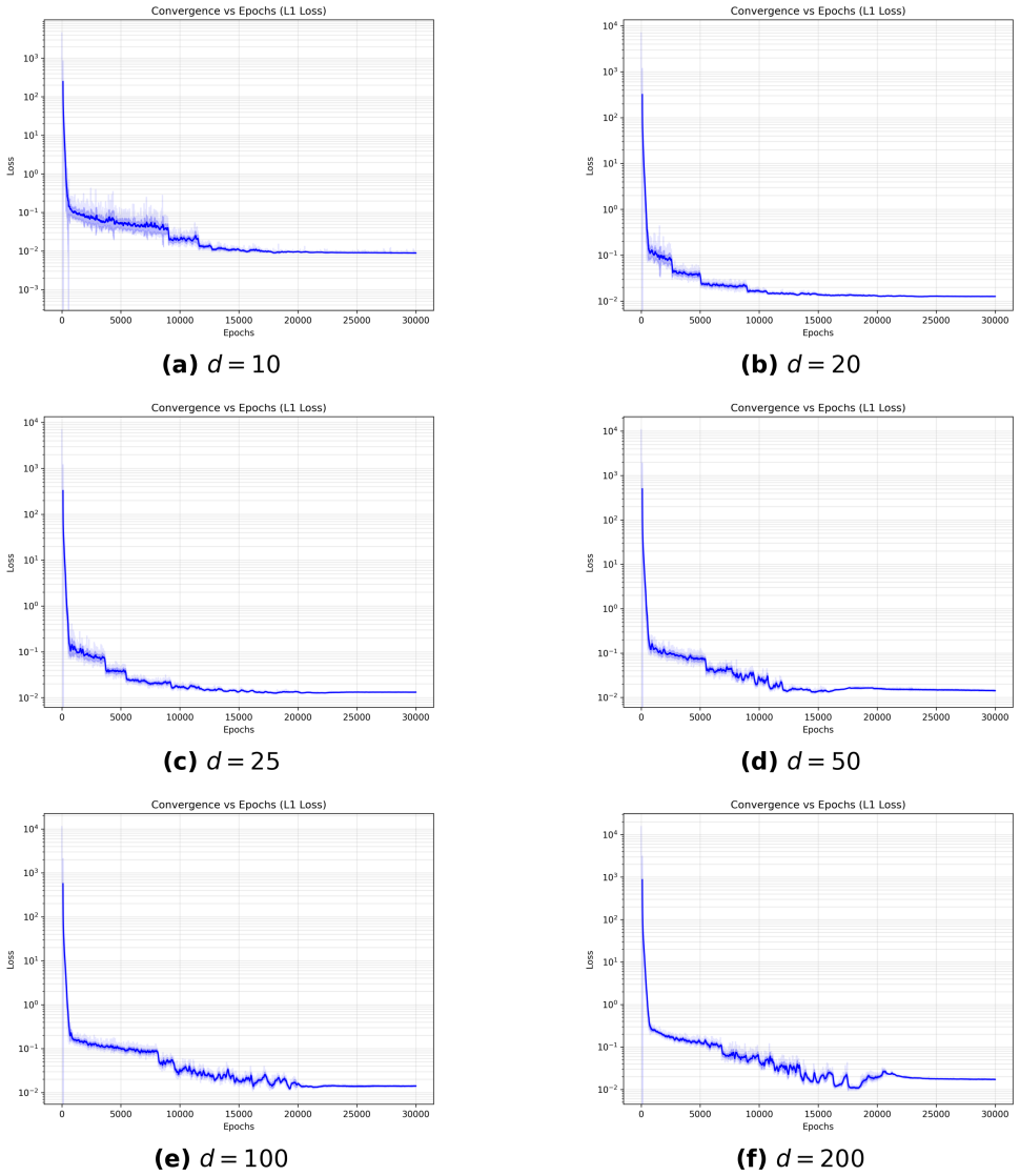
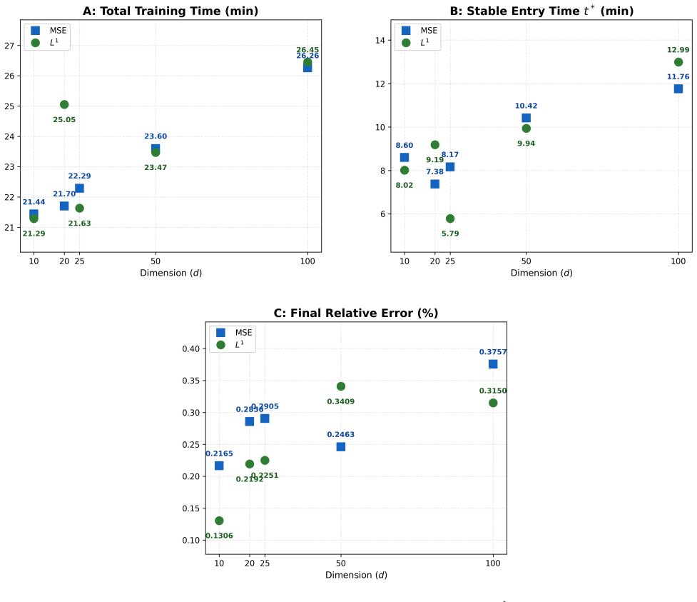
We propose a deep learning algorithm for high dimensional optimal stopping problems. Our method is inspired by the penalty method for solving free boundary PDEs. Within our approach, the penalized PDE is approximated using the Deep BSDE framework proposed by \cite{weinan2017deep}, which leads us to coin the term "Deep Penalty Method (DPM)" to refer to our algorithm. We show that the error of the DPM can be bounded by the loss function and $O(\frac{1}{\lambda})+O(\lambda h) +O(\sqrt{h})$, where $h$ is the step size in time and $\lambda$ is the penalty parameter. This finding emphasizes the need for careful consideration when selecting the penalization parameter and suggests that the discretization error converges at a rate of order $\frac{1}{2}$. We validate the efficacy of the DPM through numerical tests conducted on a high-dimensional optimal stopping model in the area of American option pricing. The numerical tests confirm both the accuracy and the computational efficiency of our proposed algorithm.
Editorial analysis
A structured set of objections, weighed in public.
Referee Report
Summary. The manuscript proposes the Deep Penalty Method (DPM) for high-dimensional optimal stopping problems. It combines the classical penalty method for free-boundary PDEs with the Deep BSDE solver of Weinan et al. (2017), states an a-priori error bound of the form training loss + O(1/λ) + O(λ h) + O(√h), and reports numerical confirmation on a high-dimensional American put pricing example.
Significance. If the error bound can be established with explicit control on the λ-dependence of the Deep BSDE approximation error, the result would supply a theoretically grounded deep-learning route to high-dimensional optimal stopping, a setting where grid-based and Monte-Carlo methods suffer from the curse of dimensionality.
major comments (2)
- [Abstract] Abstract: the claimed error bound is stated without derivation, without explicit assumptions on the Deep BSDE approximation error, and without any quantitative error tables or baseline comparisons. Because the bound is the central theoretical claim, its absence leaves the main result unsupported.
- [Abstract] Abstract: the stated combination error ≤ loss + O(1/λ) + O(λ h) + O(√h) presupposes that the Deep BSDE approximation error for the penalized PDE remains bounded independently of λ. Standard Deep BSDE analysis yields constants that grow with the Lipschitz constant of the driver; the penalty term λ max(u-g,0) makes this Lipschitz constant scale at least linearly with λ, so extra factors such as λ√h cannot be ruled out a priori.
minor comments (1)
- The numerical section should report concrete values of the training loss, the chosen λ, the observed L² or sup-norm errors, and at least one standard baseline (e.g., Longstaff–Schwartz or a plain Deep BSDE without penalty) so that the practical gain can be quantified.
Simulated Author's Rebuttal
We thank the referee for the careful reading and constructive comments. We address the major comments point by point below.
read point-by-point responses
-
Referee: [Abstract] Abstract: the claimed error bound is stated without derivation, without explicit assumptions on the Deep BSDE approximation error, and without any quantitative error tables or baseline comparisons. Because the bound is the central theoretical claim, its absence leaves the main result unsupported.
Authors: The abstract is a concise summary. The full derivation of the error bound together with the explicit assumptions on the Deep BSDE approximation error appears in Section 3. Section 4 contains numerical error tables for the high-dimensional American put. We will revise the abstract to reference the assumptions and the location of the proof, and we will add further baseline comparisons in the numerical experiments. revision: yes
-
Referee: [Abstract] Abstract: the stated combination error ≤ loss + O(1/λ) + O(λ h) + O(√h) presupposes that the Deep BSDE approximation error for the penalized PDE remains bounded independently of λ. Standard Deep BSDE analysis yields constants that grow with the Lipschitz constant of the driver; the penalty term λ max(u-g,0) makes this Lipschitz constant scale at least linearly with λ, so extra factors such as λ√h cannot be ruled out a priori.
Authors: We agree that the λ-dependence of the Deep BSDE error must be controlled explicitly. Our analysis tracks the Lipschitz constant of the penalized driver and absorbs its effect into the O(λ h) term; the resulting bound on the Deep BSDE error does not introduce additional factors of λ beyond those already stated. We will add a clarifying remark (or short appendix) that makes this control explicit. revision: partial
Circularity Check
No significant circularity; error bound is standard decomposition
full rationale
The paper derives an error bound for its DPM by combining the known penalty-method approximation error O(1/λ) + O(λ h) with the training loss of the externally cited Deep BSDE solver (Weinan et al. 2017) plus O(√h) discretization. This is a conventional a-priori bound that does not equate the final claim to its inputs by construction, nor does it rely on self-citations, fitted parameters renamed as predictions, or smuggled ansatzes. The derivation remains self-contained against the cited external framework and does not reduce the stated result to tautology.
Axiom & Free-Parameter Ledger
free parameters (2)
- penalty parameter λ
- time step h
axioms (2)
- domain assumption The Deep BSDE method of Weinan et al. (2017) can be applied directly to the penalized PDE and produces an approximation whose error combines additively with the penalty and discretization terms.
- domain assumption The solution of the penalized PDE converges to the solution of the original free-boundary problem at a rate controlled by 1/λ.
Lean theorems connected to this paper
-
IndisputableMonolith/Cost/FunctionalEquation.leanwashburn_uniqueness_aczel unclear?
unclearRelation between the paper passage and the cited Recognition theorem.
We show that the error of the DPM can be bounded by the loss function and O(1/λ)+O(λ h)+O(√h)
-
IndisputableMonolith/Foundation/ArithmeticFromLogic.leanLogicNat recovery unclear?
unclearRelation between the paper passage and the cited Recognition theorem.
the penalized PDE is approximated using the Deep BSDE framework
What do these tags mean?
- matches
- The paper's claim is directly supported by a theorem in the formal canon.
- supports
- The theorem supports part of the paper's argument, but the paper may add assumptions or extra steps.
- extends
- The paper goes beyond the formal theorem; the theorem is a base layer rather than the whole result.
- uses
- The paper appears to rely on the theorem as machinery.
- contradicts
- The paper's claim conflicts with a theorem or certificate in the canon.
- unclear
- Pith found a possible connection, but the passage is too broad, indirect, or ambiguous to say the theorem truly supports the claim.
Forward citations
Cited by 1 Pith paper
-
Two-grid Penalty Approximation Scheme for Doubly Reflected BSDEs
A two-grid penalization scheme for doubly reflected BSDEs achieves an explicit O(Δt^{1/2}) error bound when the penalty parameter λ is tuned as Δt^{-1/2} and the fine grid satisfies Δ̃t = O(Δt/λ²).
Reference graph
Works this paper leans on
-
[1]
" write newline "" before.all 'output.state := FUNCTION n.dashify 't := "" t empty not t #1 #1 substring "-" = t #1 #2 substring "--" = not "--" * t #2 global.max substring 't := t #1 #1 substring "-" = "-" * t #2 global.max substring 't := while if t #1 #1 substring * t #2 global.max substring 't := if while FUNCTION word.in bbl.in " " * FUNCTION format....
- [2]
-
[3]
Becker, S., P. Cheridito, and A. Jentzen (2019): Deep optimal stopping, Journal of Machine Learning Research, 20, 1--25
work page 2019
- [4]
-
[5]
Bouchard, B. and N. Touzi (2004): Discrete-time approximation and Monte-Carlo simulation of backward stochastic differential equations, Stochastic Processes and their applications, 111, 175--206
work page 2004
-
[6]
Broadie, M., P. Glasserman, et al. (2004): A stochastic mesh method for pricing high-dimensional American options, Journal of Computational Finance, 7, 35--72
work page 2004
-
[7]
Chan-Wai-Nam, Q., J. Mikael, and X. Warin (2019): Machine learning for semi linear PDEs, Journal of Scientific Computing, 79, 1667--1712
work page 2019
-
[8]
Chen, Y. and J. W. Wan (2021): Deep neural network framework based on backward stochastic differential equations for pricing and hedging American options in high dimensions, Quantitative Finance, 21, 45--67
work page 2021
-
[9]
E, W., J. Han, and A. Jentzen (2017): Deep learning-based numerical methods for high-dimensional parabolic partial differential equations and backward stochastic differential equations, Communications in Mathematics and Statistics, 5, 349--380
work page 2017
-
[10]
Forsyth, P. A. and K. R. Vetzal (2002): Quadratic convergence for valuing American options using a penalty method, SIAM Journal on Scientific Computing, 23, 2095--2122
work page 2002
-
[11]
Han, J., A. Jentzen, and W. E (2018): Solving high-dimensional partial differential equations using deep learning, Proceedings of the National Academy of Sciences, 115, 8505--8510
work page 2018
-
[12]
Han, J. and J. Long (2020): Convergence of the deep BSDE method for coupled FBSDEs, Probability, Uncertainty and Quantitative Risk, 5, 5
work page 2020
-
[13]
Haugh, M. B. and L. Kogan (2004): Pricing American options: A duality approach, Operations Research, 52, 258--270
work page 2004
- [14]
-
[15]
Howison, S. D., C. Reisinger, and J. H. Witte (2013): The effect of nonsmooth payoffs on the penalty approximation of American options, SIAM Journal on Financial Mathematics, 4, 539--574
work page 2013
-
[16]
(2003): Options, Futures, and Other Derivatives, Pearson, Eighth Editon
Hull, J. (2003): Options, Futures, and Other Derivatives, Pearson, Eighth Editon
work page 2003
-
[17]
Hur \'e , C., H. Pham, and X. Warin (2019): Some machine learning schemes for high-dimensional nonlinear PDEs, arXiv preprint arXiv:1902.01599, 2
-
[18]
--- -.1pt --- -.1pt --- (2020): Deep backward schemes for high-dimensional nonlinear PDEs, Mathematics of Computation, 89, 1547--1579
work page 2020
-
[19]
Jiang, L. and M. Dai (2004): Convergence of binomial tree methods for European/American path-dependent options, SIAM Journal on Numerical Analysis, 42, 1094--1109
work page 2004
-
[20]
Karatzas, I. and S. Shreve (2012): Brownian motion and stochastic calculus, vol. 113, Springer Science & Business Media
work page 2012
-
[21]
Kohler, M., A. Krzy \.z ak, and N. Todorovic (2010): Pricing of High-Dimensional American Options by Neural Networks, Mathematical Finance: An International Journal of Mathematics, Statistics and Financial Economics, 20, 383--410
work page 2010
-
[22]
Lagaris, I. E., A. Likas, and D. I. Fotiadis (1998): Artificial neural networks for solving ordinary and partial differential equations, IEEE transactions on neural networks, 9, 987--1000
work page 1998
-
[23]
Liang, G. (2015): Stochastic control representations for penalized backward stochastic differential equations, SIAM Journal on Control and Optimization, 53, 1440--1463
work page 2015
-
[24]
Liang, G., E. L \"u tkebohmert, and W. Wei (2015): Funding liquidity, debt tenor structure, and creditor’s belief: an exogenous dynamic debt run model, Mathematics and Financial Economics, 9, 271--302
work page 2015
-
[25]
Liang, G. and W. Wei (2016): Optimal switching at Poisson random intervention times, Discrete and Continuous Dynamic Systems Series B, 21, 1483--1505
work page 2016
-
[26]
Liang, J., B. Hu, L. Jiang, and B. Bian (2007): On the rate of convergence of the binomial tree scheme for American options, Numerische Mathematik, 107, 333--352
work page 2007
-
[27]
Longstaff, F. A. and E. S. Schwartz (2001): Valuing American options by simulation: a simple least-squares approach, The review of financial studies, 14, 113--147
work page 2001
-
[28]
Na, A. S. and J. W. Wan (2023): Efficient pricing and hedging of high-dimensional American options using deep recurrent networks, Quantitative Finance, 23, 631--651
work page 2023
-
[29]
Pardoux, E. and S. Peng (2005): Backward stochastic differential equations and quasilinear parabolic partial differential equations, in Stochastic Partial Differential Equations and Their Applications: Proceedings of IFIP WG 7/1 International Conference University of North Carolina at Charlotte, NC June 6--8, 1991, Springer, 200--217
work page 2005
-
[30]
Pardoux, E. and S. Tang (1999): Forward-backward stochastic differential equations and quasilinear parabolic PDEs, Probability Theory and Related Fields, 114, 123--150
work page 1999
-
[31]
(2009): Continuous-time stochastic control and optimization with financial applications, vol
Pham, H. (2009): Continuous-time stochastic control and optimization with financial applications, vol. 61, Springer Science & Business Media
work page 2009
-
[32]
Platen, E. and N. Bruti-Liberati (2010): Numerical solution of stochastic differential equations with jumps in finance, vol. 64, Springer Science & Business Media
work page 2010
-
[33]
Raissi, M. (2018): Forward-backward stochastic neural networks: Deep learning of high-dimensional partial differential equations, arXiv preprint arXiv:1804.07010
work page internal anchor Pith review Pith/arXiv arXiv 2018
-
[34]
Reisinger, C. and J. H. Witte (2012): On the use of policy iteration as an easy way of pricing American options, SIAM Journal on Financial Mathematics, 3, 459--478
work page 2012
-
[35]
Sirignano, J. and K. Spiliopoulos (2018): DGM: A deep learning algorithm for solving partial differential equations, Journal of computational physics, 375, 1339--1364
work page 2018
- [36]
-
[37]
(2013): Springer, Optimal Stochastic Control, Stochastic Target Problems, and Backwards SDE
Touzi, N. (2013): Springer, Optimal Stochastic Control, Stochastic Target Problems, and Backwards SDE
work page 2013
-
[38]
Witte, J. H. and C. Reisinger (2011): A penalty method for the numerical solution of Hamilton--Jacobi--Bellman (HJB) equations in finance, SIAM Journal on Numerical Analysis, 49, 213--231
work page 2011
discussion (0)
Sign in with ORCID, Apple, or X to comment. Anyone can read and Pith papers without signing in.