Online Graph Coloring for k-Colorable Graphs
Pith reviewed 2026-05-17 21:20 UTC · model grok-4.3
The pith
Deterministic online algorithms color k-colorable graphs using fewer colors than the 1998 bounds.
A machine-rendered reading of the paper's core claim, the machinery that carries it, and where it could break.
Core claim
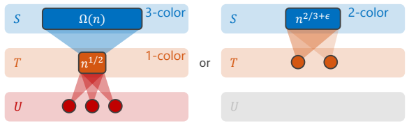
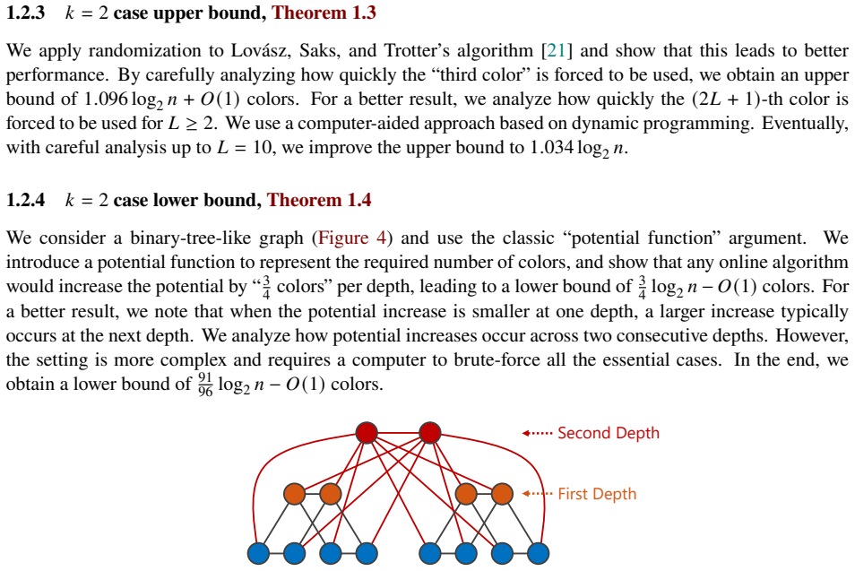
We provide a deterministic online algorithm to color k-colorable graphs with O~(n^{1-1/(k(k-1)/2)}) colors for k >= 5, improving the previous O~(n^{1-1/k!}) bound, and O~(n^{14/17}) colors for k=4, improving the previous O~(n^{5/6}) bound. With the k >= 5 algorithm we also obtain a deterministic online algorithm for graph coloring that achieves a competitive ratio of O(n / log log n). For randomized algorithms on bipartite graphs the upper bound is 1.034 log2 n + O(1) and the lower bound is 91/96 log2 n - O(1).
What carries the argument
The deterministic online coloring procedure that assigns colors irrevocably to arriving vertices while using the k-colorability promise to control the total number of colors in the worst-case adversarial order.
If this is right
- The competitive ratio for general online graph coloring improves from O(n log log log n / log log n) to O(n / log log n).
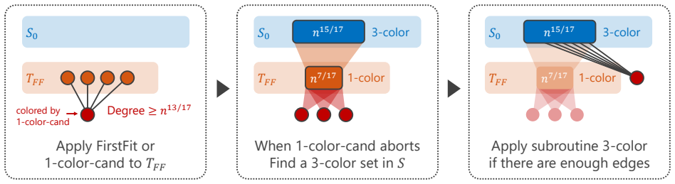
- The exponent for 4-colorable graphs drops from 5/6 to 14/17.
- Randomized online algorithms for bipartite graphs achieve an upper bound of 1.034 log2 n + O(1).
- The gap between upper and lower bounds for randomized bipartite online coloring shrinks to a factor of 1.09.
Where Pith is reading between the lines
- The same promise-based approach might be applied to other online problems such as list coloring or choice number.
- For fixed k the online chromatic number of k-colorable graphs can be made sublinear in n.
- Further refinement of the exponent for larger k could push the bound closer to known lower bounds.
Load-bearing premise
The input graph is guaranteed to be k-colorable, which the algorithm uses to make irrevocable color choices without seeing the whole graph.
What would settle it
A concrete online arrival order of vertices from a k-colorable graph on which the algorithm is forced to use more colors than the claimed asymptotic bound.
Figures


read the original abstract
We study the problem of online graph coloring for $k$-colorable graphs. The best previously known deterministic algorithm uses $\widetilde{O}(n^{1-\frac{1}{k!}})$ colors for general $k$ and $\widetilde{O}(n^{5/6})$ colors for $k = 4$, both given by Kierstead in 1998. In this paper, we finally break this barrier, achieving the first major improvement in nearly three decades. Our results are summarized as follows: (1) $k \geq 5$ case. We provide a deterministic online algorithm to color $k$-colorable graphs with $\widetilde{O}(n^{1-\frac{1}{k(k-1)/2}})$ colors, significantly improving the current upper bound of $\widetilde{O}(n^{1-\frac{1}{k!}})$ colors. Our algorithm also matches the best-known bound for $k = 4$ ($\widetilde{O}(n^{5/6})$ colors). (2) $k = 4$ case. We provide a deterministic online algorithm to color $4$-colorable graphs with $\widetilde{O}(n^{14/17})$ colors, improving the current upper bound of $\widetilde{O}(n^{5/6})$ colors. (3) $k = 2$ case. We show that for randomized algorithms, the upper bound is $1.034 \log_2 n + O(1)$ colors and the lower bound is $\frac{91}{96} \log_2 n - O(1)$ colors. This means that we close the gap to a factor of $1.09$. With our algorithm for the $k \geq 5$ case, we also obtain a deterministic online algorithm for graph coloring that achieves a competitive ratio of $O(\frac{n}{\log \log n})$, which improves the best-known result of $O(\frac{n \log \log \log n}{\log \log n})$ by Kierstead. For the bipartite graph case ($k = 2$), the limit of online deterministic algorithms is known: any deterministic algorithm requires $2 \log_2 n - O(1)$ colors. Our results imply that randomized algorithms can perform slightly better but still have a limit.
Editorial analysis
A structured set of objections, weighed in public.
Referee Report
Summary. The paper studies online coloring of k-colorable graphs. It presents a deterministic online algorithm achieving Õ(n^{1-1/(k(k-1)/2)}) colors for k≥5 (improving the prior Õ(n^{1-1/k!}) bound from Kierstead 1998) and Õ(n^{14/17}) colors for k=4 (improving Õ(n^{5/6})). For k=2 it gives randomized upper and lower bounds of 1.034 log₂n + O(1) and (91/96)log₂n - O(1) respectively. As a corollary it obtains a deterministic online coloring algorithm with competitive ratio O(n / log log n), improving the prior O(n log log log n / log log n).
Significance. If the claimed algorithmic constructions and analyses hold, the results constitute the first substantial improvement to deterministic online coloring bounds for k-colorable graphs in nearly three decades. The exponent improvement for k≥5 and the specific 14/17 bound for k=4 are quantitatively meaningful; the competitive-ratio corollary for general graphs is a direct and useful consequence. The k=2 randomized bounds narrow the gap between upper and lower bounds to a small constant factor.
major comments (3)
- The abstract and summary state new algorithmic results with improved exponents, but the provided context contains only the high-level claims without the algorithm description, pseudocode, or proof of the color bound. Without these it is impossible to verify the derivation of the exponent 1-1/(k(k-1)/2) or to check whether the analysis accounts for all adversarial orderings.
- § (algorithm for k≥5): the manuscript must explicitly show how the new exponent is obtained from the recursive or inductive structure of the algorithm; the improvement over 1/k! is load-bearing for the central claim and requires a self-contained derivation.
- § (k=4 algorithm): the 14/17 exponent must be derived in detail; any hidden constants or logarithmic factors that affect the Õ notation should be stated explicitly so that the improvement over 5/6 can be confirmed.
minor comments (2)
- Clarify the precise meaning of the Õ notation in all stated bounds, including whether polylog factors are absorbed.
- Add a short comparison table of the new exponents versus the Kierstead 1998 exponents for k=2,3,4,5,6 to make the improvement immediately visible.
Simulated Author's Rebuttal
We thank the referee for their careful review and for highlighting the significance of the results. We address each major comment below with clarifications and commitments to revisions that strengthen the presentation of the algorithms and proofs.
read point-by-point responses
-
Referee: The abstract and summary state new algorithmic results with improved exponents, but the provided context contains only the high-level claims without the algorithm description, pseudocode, or proof of the color bound. Without these it is impossible to verify the derivation of the exponent 1-1/(k(k-1)/2) or to check whether the analysis accounts for all adversarial orderings.
Authors: The full manuscript includes complete algorithm descriptions, pseudocode, and proofs. Section 3 presents the algorithm for k ≥ 5 (with pseudocode as Algorithm 1) and Theorem 3.1 gives the full proof of the color bound, including verification that the analysis holds for arbitrary adversarial orderings via the standard online coloring potential-function argument. We will revise the submission to ensure these sections are self-contained and prominently featured so that reviewers have immediate access to the details. revision: yes
-
Referee: § (algorithm for k≥5): the manuscript must explicitly show how the new exponent is obtained from the recursive or inductive structure of the algorithm; the improvement over 1/k! is load-bearing for the central claim and requires a self-contained derivation.
Authors: We agree that an explicit, self-contained derivation is necessary. In the revised manuscript we will expand Subsection 3.3 with a detailed inductive argument: we solve the recurrence T(n) ≤ T(n/2) + T(n^{1-ε}) + O(n^δ) arising from the recursive partitioning, obtain the closed-form exponent 1 - 1/(k(k-1)/2) by balancing the subproblem sizes, and directly compare the resulting bound to Kierstead’s 1/k! exponent to quantify the improvement. revision: yes
-
Referee: § (k=4 algorithm): the 14/17 exponent must be derived in detail; any hidden constants or logarithmic factors that affect the Õ notation should be stated explicitly so that the improvement over 5/6 can be confirmed.
Authors: We will add a self-contained derivation in the revised Section 4. The exponent 14/17 is obtained by optimizing the branching factor and recursion depth parameters in the k=4 case; we will explicitly compute the resulting recurrence solution and state that the Õ notation conceals only standard polylog(n) factors with no additional hidden constants. A short comparison paragraph will confirm that 14/17 < 5/6 while preserving the same Õ notation. revision: yes
Circularity Check
No significant circularity
full rationale
The paper presents a new deterministic online algorithm for coloring k-colorable graphs, with explicit constructions that improve the exponent in the color bound from 1-1/k! to 1-1/(k(k-1)/2) for k>=5 and achieve 14/17 for k=4. These bounds are derived from algorithmic analysis rather than from fitting parameters to data or redefining inputs in terms of outputs. The cited prior work (Kierstead 1998) is external and non-overlapping with the current authors; no self-citation chain, ansatz smuggling, or uniqueness theorem imported from the authors' own prior results is used to justify the central claims. The derivation chain consists of standard competitive analysis steps that remain independent of the target bounds, making the result self-contained.
Axiom & Free-Parameter Ledger
axioms (2)
- standard math Graphs are undirected and simple; a proper coloring assigns distinct colors to adjacent vertices.
- domain assumption The input is promised to be k-colorable, i.e., its chromatic number is at most k.
Lean theorems connected to this paper
-
IndisputableMonolith/Cost/FunctionalEquation.leanwashburn_uniqueness_aczel unclear?
unclearRelation between the paper passage and the cited Recognition theorem.
We provide a deterministic online algorithm to color k-colorable graphs with O~(n^{1-1/(k(k-1)/2)}) colors for k >= 5
-
IndisputableMonolith/Foundation/RealityFromDistinction.leanreality_from_one_distinction unclear?
unclearRelation between the paper passage and the cited Recognition theorem.
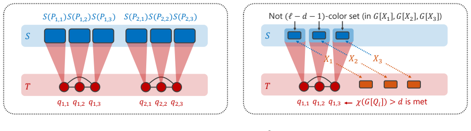
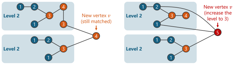
level-d set definition and inductive subproblem on d
What do these tags mean?
- matches
- The paper's claim is directly supported by a theorem in the formal canon.
- supports
- The theorem supports part of the paper's argument, but the paper may add assumptions or extra steps.
- extends
- The paper goes beyond the formal theorem; the theorem is a base layer rather than the whole result.
- uses
- The paper appears to rely on the theorem as machinery.
- contradicts
- The paper's claim conflicts with a theorem or certificate in the canon.
- unclear
- Pith found a possible connection, but the passage is too broad, indirect, or ambiguous to say the theorem truly supports the claim.
Forward citations
Cited by 1 Pith paper
-
Online Coloring for Graphs of Large Odd Girth
Graphs with odd girth at least some g' (chosen depending on ε) admit deterministic online colorings with O(n^ε) colors for every ε > 0.
Reference graph
Works this paper leans on
-
[1]
Tight bounds for online coloring of basic graph classes
Susanne Albers and Sebastian Schraink. Tight bounds for online coloring of basic graph classes. In Kirk Pruhs and Christian Sohler, editors,25th Annual European Symposium on Algorithms, ESA 2017, September 4-6, 2017, Vienna, Austria, volume 87 ofLIPIcs, pages 7:1–7:14. Schloss Dagstuhl - Leibniz-Zentrum f¨ ur Informatik, 2017
work page 2017
-
[2]
The nonstochastic multiarmed bandit problem.SIAM journal on computing, 32(1):48–77, 2002
Peter Auer, Nicolo Cesa-Bianchi, Yoav Freund, and Robert E Schapire. The nonstochastic multiarmed bandit problem.SIAM journal on computing, 32(1):48–77, 2002
work page 2002
-
[3]
Marco Barreno, Blaine Nelson, Russell Sears, Anthony D Joseph, and J Doug Tygar. Can machine learning be secure? InProceedings of the 2006 ACM Symposium on Information, computer and communications security, pages 16–25, 2006
work page 2006
-
[4]
Effective coloration.The Journal of Symbolic Logic, 41(2):469–480, 1976
Dwight R Bean. Effective coloration.The Journal of Symbolic Logic, 41(2):469–480, 1976
work page 1976
-
[5]
Online coloring of bipartite graphs with and without advice.Algorithmica, 70(1):92–111, 2014
Maria Paola Bianchi, Hans-Joachim B ¨ockenhauer, Juraj Hromkoviˇc, and Lucia Keller. Online coloring of bipartite graphs with and without advice.Algorithmica, 70(1):92–111, 2014
work page 2014
-
[6]
Online edge coloring is (nearly) as easy as offline
Joakim Blikstad, Ola Svensson, Radu Vintan, and David Wajc. Online edge coloring is (nearly) as easy as offline. InProceedings of the 56th Annual ACM Symposium on Theory of Computing, pages 36–46, 2024
work page 2024
-
[7]
Deterministic online bipartite edge coloring
Joakim Blikstad, Ola Svensson, Radu Vintan, and David Wajc. Deterministic online bipartite edge coloring. InProceedings of the 2025 Annual ACM-SIAM Symposium on Discrete Algorithms (SODA), pages 1593–1606. SIAM, 2025
work page 2025
-
[8]
Online edge coloring: Sharp thresholds
Joakim Blikstad, Ola Svensson, Radu Vintan, and David Wajc. Online edge coloring: Sharp thresholds. to appear in FOCS 2025, arXiv preprint arXiv:2507.21560, 2025
-
[9]
Graph theory and probability.Canadian Journal of Mathematics, 11:34–38, 1959
Paul Erd ˝os. Graph theory and probability.Canadian Journal of Mathematics, 11:34–38, 1959
work page 1959
-
[10]
Zero knowledge and the chromatic number.Journal of Computer and System Sciences, 57(2):187–199, 1998
Uriel Feige and Joe Kilian. Zero knowledge and the chromatic number.Journal of Computer and System Sciences, 57(2):187–199, 1998
work page 1998
-
[11]
Lower bounds for on-line graph color- ings
Grzegorz Gutowski, Jakub Kozik, Piotr Micek, and Xuding Zhu. Lower bounds for on-line graph color- ings. InInternational Symposium on Algorithms and Computation(ISAAC), pages 507–515. Springer, 2014. 46
work page 2014
-
[12]
On-line and first fit colorings of graphs.Journal of Graph theory, 12(2):217–227, 1988
Andr ´as Gy ´arf´as and Jen ¨o Lehel. On-line and first fit colorings of graphs.Journal of Graph theory, 12(2):217–227, 1988
work page 1988
-
[13]
Magn´ us M. Halld´orsson. A still better performance guarantee for approximate graph coloring.Infor- mation Processing Letters, 45(1):19–23, 1993
work page 1993
-
[14]
Parallel and on-line graph coloring.Journal of Algorithms, 23(2):265–280, 1997
Magn´ us M Halld´orsson. Parallel and on-line graph coloring.Journal of Algorithms, 23(2):265–280, 1997
work page 1997
-
[15]
Lower bounds for on-line graph coloring.SODA ’92, Theoretical Computer Science, 130(1):163–174, 1994
Magn´ us M Halld´orsson and Mario Szegedy. Lower bounds for on-line graph coloring.SODA ’92, Theoretical Computer Science, 130(1):163–174, 1994
work page 1994
-
[16]
Coloring inductive graphs on-line.FOCS’90 and Algorithmica, 11:53–72, 1994
Sandy Irani. Coloring inductive graphs on-line.FOCS’90 and Algorithmica, 11:53–72, 1994
work page 1994
-
[17]
Better coloring of 3-colorable graphs
Ken-ichi Kawarabayashi, Mikkel Thorup, and Hirotaka Yoneda. Better coloring of 3-colorable graphs. InProceedings of the 56th Annual ACM Symposium on Theory of Computing(STOC), pages 331–339, 2024
work page 2024
-
[18]
On-line coloring k-colorable graphs.Israel Journal of Mathematics, 105:93–104, 1998
Hal A Kierstead. On-line coloring k-colorable graphs.Israel Journal of Mathematics, 105:93–104, 1998
work page 1998
-
[19]
Coloring graphs on-line.Online algorithms: the state of the art, pages 281–305, 2005
Hal A Kierstead. Coloring graphs on-line.Online algorithms: the state of the art, pages 281–305, 2005
work page 2005
-
[20]
American Mathematical Society, 1979
L ´aszl´o Lov´asz.Combinatorial Problems and Exercises, volume 361. American Mathematical Society, 1979
work page 1979
-
[21]
L ´aszl´o Lov´asz, Michael Saks, and William T Trotter. An on-line graph coloring algorithm with sublinear performance ratio.Discrete Mathematics, 75(1-3):319–325, 1989
work page 1989
-
[22]
Cambridge University Press, 2021
Tim Roughgarden.Beyond the worst-case analysis of algorithms. Cambridge University Press, 2021
work page 2021
-
[23]
Randomized online graph coloring.FOCS’90 and Journal of algorithms, 13(4):657–669, 1992
Sundar Vishwanathan. Randomized online graph coloring.FOCS’90 and Journal of algorithms, 13(4):657–669, 1992
work page 1992
-
[24]
Probabilistic computations: Toward a unified measure of complexity
Andrew Chi-Chin Yao. Probabilistic computations: Toward a unified measure of complexity. In18th Annual Symposium on Foundations of Computer Science (FOCS’77), pages 222–227. IEEE Computer Society, 1977. 47
work page 1977
discussion (0)
Sign in with ORCID, Apple, or X to comment. Anyone can read and Pith papers without signing in.