Does "Do Differentiable Simulators Give Better Policy Gradients?'' Give Better Policy Gradients?
Pith reviewed 2026-05-10 05:20 UTC · model grok-4.3
The pith
Variance control in gradient estimators often outperforms explicit discontinuity detection when using differentiable simulators for policy gradients.
A machine-rendered reading of the paper's core claim, the machinery that carries it, and where it could break.
Core claim
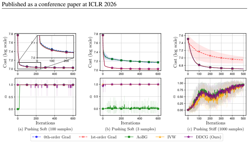
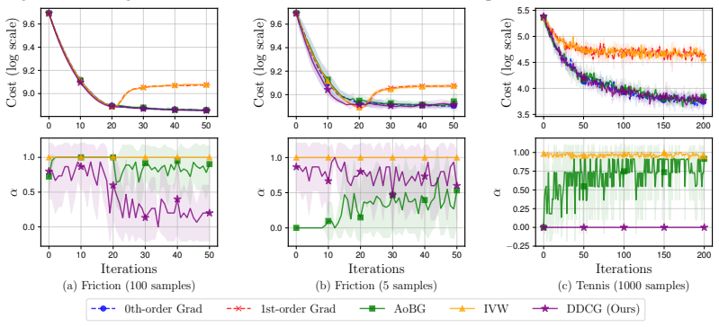
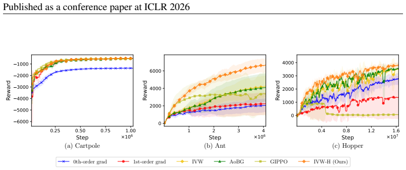
Access to differentiable models enables first-order policy gradient estimates that can accelerate learning, yet discontinuities introduce bias that undermines them. Prior detection methods using REINFORCE confidence intervals suffer from high noise and low efficiency. Re-examination reveals that a lightweight switching test called DDCG, using a single hyperparameter, achieves robust results in discontinuous settings even with small sample sizes. Separately, on differentiable robotics tasks, per-step inverse-variance weighting (IVW-H) stabilizes estimates without any discontinuity detection and delivers strong performance, suggesting variance control is often more important than explicit bias
What carries the argument
DDCG, a discontinuity detection and gradient estimator switching method with one hyperparameter, and IVW-H, a per-step inverse-variance weighting scheme for stabilizing first-order gradients.
If this is right
- DDCG provides robust performance in standard discontinuous test settings using minimal tuning and small samples.
- IVW-H yields strong results on differentiable robotics control tasks without needing to detect discontinuities.
- Estimator switching improves robustness in controlled studies of non-smooth dynamics.
- Careful variance control dominates estimator performance in practical policy gradient deployments.
Where Pith is reading between the lines
- Real-world applications may benefit more from variance reduction techniques than from sophisticated discontinuity handling.
- Hybrid methods combining switching and variance weighting could be explored for even better results.
- The findings may generalize to other reinforcement learning domains with mixed smooth and non-smooth dynamics.
Load-bearing premise
That the discontinuous settings re-examined and the differentiable robotics tasks used are representative of the main challenges faced in real-world policy gradient optimization.
What would settle it
A new experiment on a discontinuous dynamics task where DDCG fails to outperform standard methods, or a robotics task where IVW-H does not stabilize gradients despite differentiability.
Figures


read the original abstract
In policy gradient reinforcement learning, access to a differentiable model enables 1st-order gradient estimation that accelerates learning compared to relying solely on derivative-free 0th-order estimators. However, discontinuous dynamics cause bias and undermine the effectiveness of 1st-order estimators. Prior work addressed this bias by constructing a confidence interval around the REINFORCE 0th-order gradient estimator and using these bounds to detect discontinuities. However, the REINFORCE estimator is notoriously noisy, and we find that this method requires task-specific hyperparameter tuning and has low sample efficiency. This paper asks whether such bias is the primary obstacle and what minimal fixes suffice. First, we re-examine standard discontinuous settings from prior work and introduce DDCG, a lightweight test that switches estimators in nonsmooth regions; with a single hyperparameter, DDCG achieves robust performance and remains reliable with small samples. Second, on differentiable robotics control tasks, we present IVW-H, a per-step inverse-variance implementation that stabilizes variance without explicit discontinuity detection and yields strong results. Together, these findings indicate that while estimator switching improves robustness in controlled studies, careful variance control often dominates in practical deployments.
Editorial analysis
A structured set of objections, weighed in public.
Referee Report
Summary. The paper questions whether bias induced by discontinuities in differentiable simulators is the primary obstacle to effective policy gradients in reinforcement learning. It re-examines standard discontinuous environments from prior work and introduces DDCG, a lightweight estimator-switching test that uses a single hyperparameter to switch between 1st-order and 0th-order gradients in nonsmooth regions. On differentiable robotics control tasks, it presents IVW-H, a per-step inverse-variance weighting scheme that stabilizes gradients without explicit discontinuity detection. The central finding is that estimator switching improves robustness in controlled studies, but careful variance control often dominates in practical deployments.
Significance. If the empirical results hold under broader testing, the work would usefully redirect attention in differentiable simulation-based RL from complex bias-correction mechanisms toward simpler, per-step variance-reduction techniques. The minimal-hyperparameter character of DDCG and the per-step formulation of IVW-H could lower barriers to adoption in robotics control pipelines where sample efficiency remains the dominant constraint.
major comments (2)
- [§4] §4 (Differentiable robotics tasks): the claim that IVW-H 'stabilizes variance without explicit discontinuity detection and yields strong results' is load-bearing for the conclusion that variance control dominates; however, the manuscript provides no quantitative comparison of variance reduction achieved by IVW-H versus standard baselines (e.g., REINFORCE with baseline or SVRG-style methods) on the same tasks, leaving open whether the reported gains are attributable to variance control or to other unstated implementation details.
- [§3] §3 (DDCG definition): the single-hyperparameter switching rule is presented as robust with small samples, yet the decision threshold appears to be tuned on the same discontinuous environments used for evaluation; without a held-out validation protocol or sensitivity analysis across a wider range of discontinuity strengths, the reported robustness may not generalize beyond the re-examined prior-work settings.
minor comments (2)
- The abstract and introduction use 'estimator switching' and 'variance control' without a concise side-by-side definition; a short table contrasting DDCG, IVW-H, and the prior confidence-interval method would improve readability.
- Notation for the inverse-variance weights in IVW-H is introduced without an explicit equation number; adding an equation label would facilitate later cross-references in the experimental discussion.
Simulated Author's Rebuttal
We thank the referee for the constructive and detailed feedback. The comments highlight important aspects of empirical validation that we will strengthen in revision. We address each major comment below.
read point-by-point responses
-
Referee: [§4] §4 (Differentiable robotics tasks): the claim that IVW-H 'stabilizes variance without explicit discontinuity detection and yields strong results' is load-bearing for the conclusion that variance control dominates; however, the manuscript provides no quantitative comparison of variance reduction achieved by IVW-H versus standard baselines (e.g., REINFORCE with baseline or SVRG-style methods) on the same tasks, leaving open whether the reported gains are attributable to variance control or to other unstated implementation details.
Authors: We agree that a direct quantitative comparison of variance reduction is needed to isolate the contribution of IVW-H. In the revised manuscript we will add gradient-variance plots and tables comparing IVW-H against REINFORCE with baseline and SVRG-style estimators on the same differentiable robotics tasks. These additions will clarify whether the observed performance gains are attributable to per-step inverse-variance weighting rather than other implementation choices. revision: yes
-
Referee: [§3] §3 (DDCG definition): the single-hyperparameter switching rule is presented as robust with small samples, yet the decision threshold appears to be tuned on the same discontinuous environments used for evaluation; without a held-out validation protocol or sensitivity analysis across a wider range of discontinuity strengths, the reported robustness may not generalize beyond the re-examined prior-work settings.
Authors: The referee is correct that the threshold was informed by the evaluation environments. We will add a sensitivity analysis that varies discontinuity strength over a wider range and include a simple held-out validation protocol in the revised manuscript. These experiments will demonstrate that the single-hyperparameter rule remains reliable beyond the original settings while preserving the lightweight character of DDCG. revision: yes
Circularity Check
No significant circularity in empirical claims or method proposals
full rationale
The paper's core contribution consists of re-examining existing discontinuous environments, proposing DDCG for estimator switching, and IVW-H for variance stabilization on robotics tasks. These are presented as lightweight empirical fixes positioned against external prior results on REINFORCE-based discontinuity detection. No equations, derivations, or predictions are shown to reduce by construction to fitted parameters, self-defined quantities, or load-bearing self-citations. The findings rest on experimental outcomes from standard benchmarks that remain independently testable outside the paper's own fitted values or assumptions.
Axiom & Free-Parameter Ledger
Reference graph
Works this paper leans on
-
[1]
11 Published as a conference paper at ICLR 2026 C Daniel Freeman, Erik Frey, Anton Raichuk, Sertan Girgin, Igor Mordatch, and Olivier Bachem. Brax–a differentiable physics engine for large scale rigid body simulation.arXiv preprint arXiv:2106.13281,
-
[2]
Analytical derivatives of rigid body dynamics algorithms
Justin Carpentier and Nicolas Mansard. Analytical derivatives of rigid body dynamics algorithms. In Robotics: Science and systems (RSS 2018),
work page 2018
-
[3]
arXiv preprint arXiv:2103.16021 (2021)
Keenon Werling, Dalton Omens, Jeongseok Lee, Ioannis Exarchos, and C Karen Liu. Fast and feature-complete differentiable physics for articulated rigid bodies with contact.arXiv preprint arXiv:2103.16021,
-
[4]
Eliot Xing, Vernon Luk, and Jean Oh. Stabilizing reinforcement learning in differentiable multiphysics simulation.arXiv preprint arXiv:2412.12089,
-
[5]
Clemens Schwarke, Victor Klemm, Jesus Tordesillas, Jean-Pierre Sleiman, and Marco Hutter. Learn- ing quadrupedal locomotion via differentiable simulation.arXiv preprint arXiv:2404.02887,
-
[6]
DODIFFERENTIABLESIMULATORSGIVEBETTER POLICYGRADIENTS?
12 Published as a conference paper at ICLR 2026 APPENDICES: DOES“DODIFFERENTIABLESIMULATORSGIVEBETTER POLICYGRADIENTS?” GIVEBETTERPOLICYGRADIENTS? A Extended Related Works 14 B Infinite Variance Example 14 C Proofs 15 D Variance of the AoBG vs. DDCG Test Statistics 17 E Pseudocode for IVW-H 19 F Function Optimization Tasks 20 G Additional Experiments 21 G...
work page 2026
-
[7]
alleviates stiffness in complementarity- based contact models by adding barrier-smoothed objectives with an adaptive central-path parameter, jointly controlling gradient variance and bias for stable 1st-order policy gradients. By smoothing contact interactions, analytic-gradient methods such as SHAC have been applied successfully to learn physically plaus...
work page 2024
-
[8]
(23) Define ∆xy =∥∇f(x)− ∇f(y)∥ 2 −L∥x−y∥ 2.(24) Noting that 2V[x] =E ∥x−y∥ 2 2 ,(25) for arbitrary random variables, we can construct another equation involving the gradient differences and the above definition: 2V ∇f(x) =E ∥∇f(x)− ∇f(y)∥ 2 2 =E (L∥x−y∥ 2 + ∆xy)2 =L 2 E ∥x−y∥ 2 2 +E ∆2 xy + 2LE ∥x−y∥ 2∆xy | {z } =0from Eq. (23) . (26) Using Eq. (25) agai...
work page 2026
-
[9]
= Θ(d 2).(40) DDCG statistic.DefineZ= ˆV[f(x)] σ2 =f(x) 2/σ2. Becausef(x)∼ N 0, dσ 2 , E[Z] =d,V[Z] = 2d 2.(41) For a batch of sizenthe statistic used by DDCG is the sample mean ˆv= 1 n nX k=1 Zk.(42) Its sampling variance is therefore V[ˆv] = V[Z] n = 2d2 n .(43) 17 Published as a conference paper at ICLR 2026 Relative precision (coefficient of variation...
work page 2026
-
[10]
Apply clipping if needed and updateθwith Adam
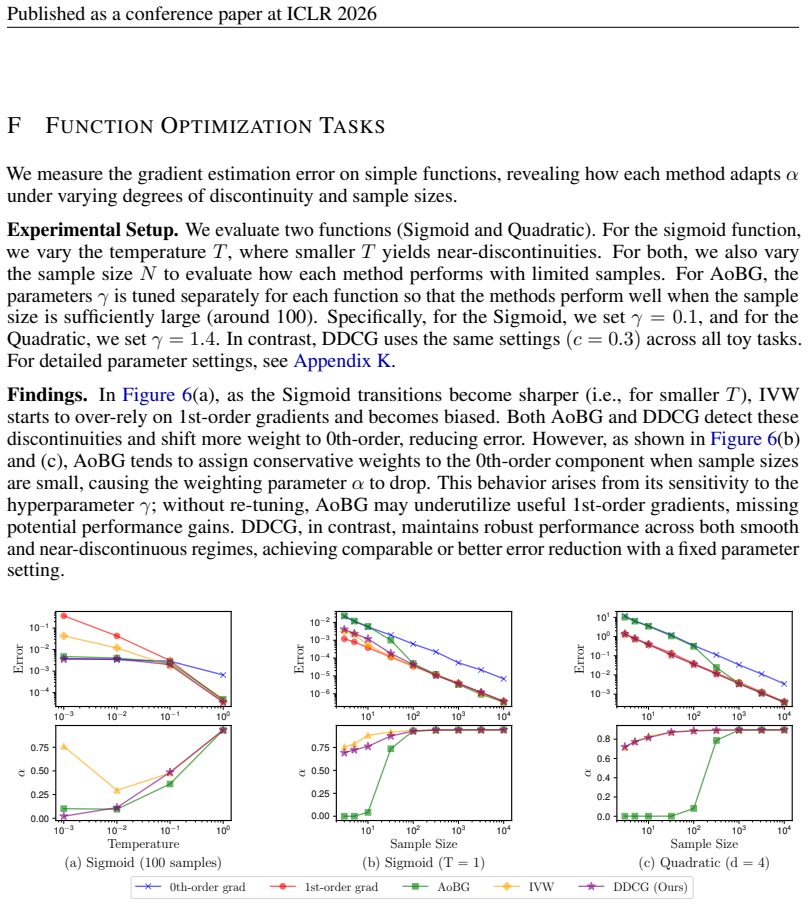
8: Push to policy weights.Treat {Gt,n,a,ϕ} as the target gradient on distribution parameters and perform a vector–Jacobian product through πθ to obtain ∇θL. Apply clipping if needed and updateθwith Adam. 9:Critic.Fit ˆVby MSE to targetsA t + ˆV(s t). 19 Published as a conference paper at ICLR 2026 F FUNCTIONOPTIMIZATIONTASKS We measure the gradient estima...
work page 2026
-
[11]
Top row: estimation errors (log scale) between true and estimated gradients for each method
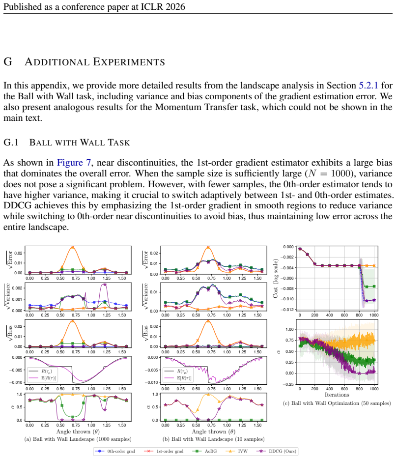
functions under varying temperatures and sample sizes. Top row: estimation errors (log scale) between true and estimated gradients for each method. Bottom row: weighting parameter α for each method, showing selection between 0th- and 1st-order gradients. 20 Published as a conference paper at ICLR 2026 G ADDITIONALEXPERIMENTS In this appendix, we provide m...
work page 2026
-
[12]
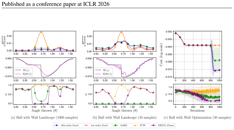
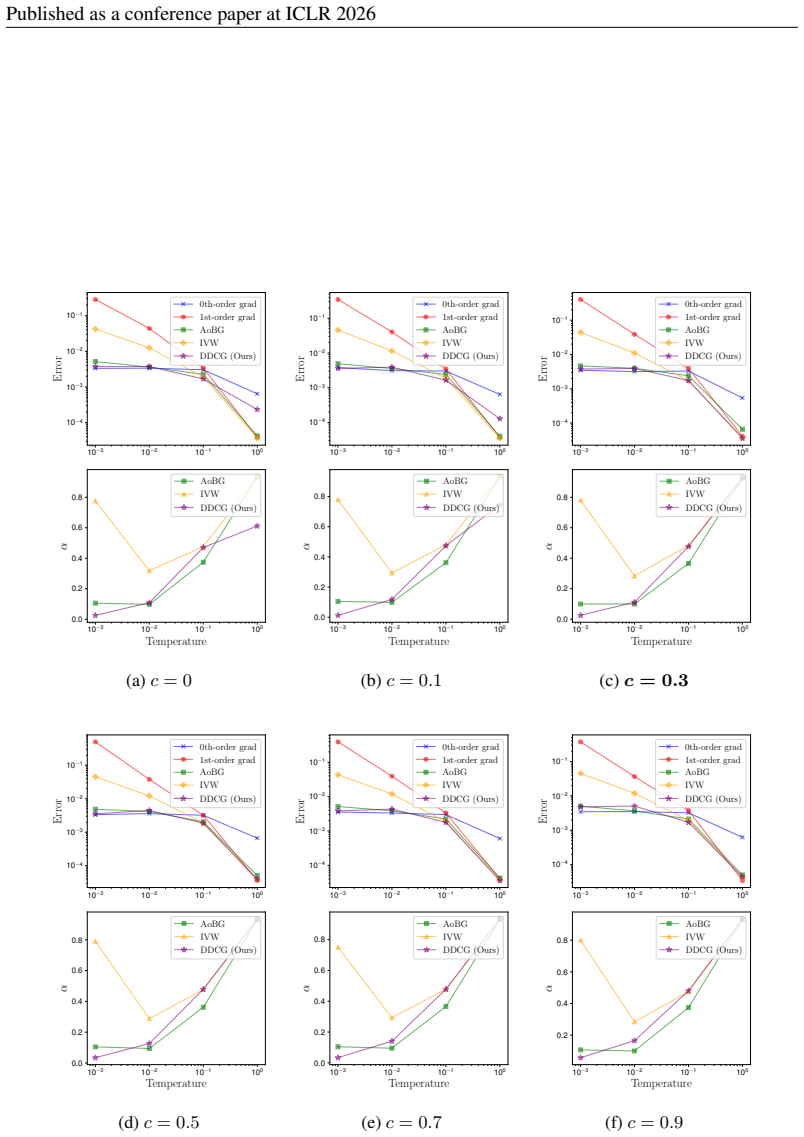
Recall that c= 1 means our test condition is always satisfied, so the method consistently applies IVW, disabling discontinuity detection. Conversely, c= 0 imposes a strong smoothness assumption, frequently falling back to the 0th-order estimator and leading to more conservative updates. For any c̸= 1 , the largest cost change near θ= 0.7 is reliably detec...
work page 2026
-
[13]
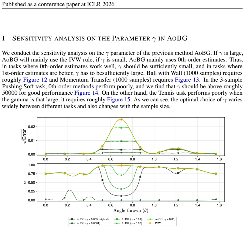
As we can see, the optimal choice of γ varies widely between different tasks and also changes with the sample size. Figure 12: Sensitivity analysis on the parameter γ for AoBG in the Ball with Wall landscape analysis (1000 samples). The figure shows the error for each input angle θ and the corresponding α selection. 0.0 0.2 0.4 0.6 0.8 1.0 1.2 1.4 1.6 0.0...
work page 2026
-
[14]
AoBG ( γ = 10000) AoBG ( γ = 100000) AoBG ( γ = 1000000) IVW (a) Ant (High-contact scenario) 0.00 0.25 0.50 0.75 1.00 1.25 1.50 Step ×107 0 500 1000 1500 2000 2500 3000 3500Reward 0.00 0.25 0.50 0.75 1.00 1.25 1.50 Step ×107 0.0 0.2 0.4 0.6 0.8 1.0 α AoBG ( γ =
work page 2000
-
[15]
We compare AoBG with varying γ against the IVW baseline
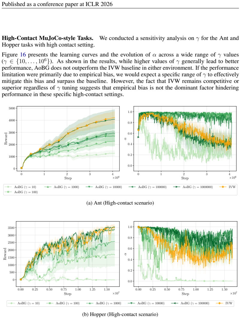
AoBG ( γ = 10000) AoBG ( γ = 100000) IVW (b) Hopper (High-contact scenario) Figure 16:Sensitivity analysis on the parameter γ for AoBG in high-contact environments. We compare AoBG with varying γ against the IVW baseline. The left plots show the learning curves (Reward), and the right plots show the evolution of the mixing coefficientα. Notably, even with...
work page 2026
discussion (0)
Sign in with ORCID, Apple, or X to comment. Anyone can read and Pith papers without signing in.