Curvature of optimal transport with respect to the cost and applications to inverse optimal transport
Pith reviewed 2026-05-08 10:56 UTC · model grok-4.3
The pith
Smooth positive densities make the optimal transport functional strictly curved with respect to the ground cost.
A machine-rendered reading of the paper's core claim, the machinery that carries it, and where it could break.
Core claim
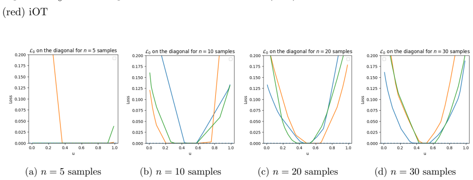
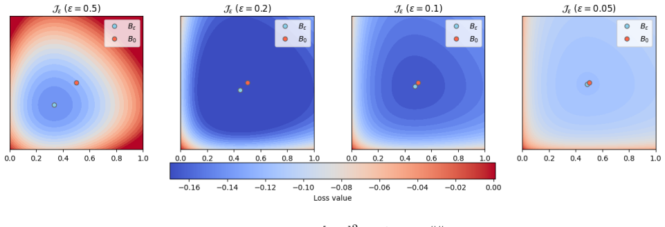
Assuming smooth positive densities for the source and target measures, we characterize the second variation of the optimal transport functional with respect to the ground cost in Hölder spaces. In particular, we show that it is non-degenerate modulo the natural transport invariances, yielding a strict curvature property that is absent in discrete transport. As a consequence, we obtain local identifiability and stability results for inverse optimal transport. For the structured family of bilinear costs, the ground cost can be uniquely recovered up to the intrinsic invariances from a single optimal coupling under a natural spanning condition.
What carries the argument
The second variation of the optimal transport functional with respect to the ground cost, characterized in Hölder spaces and proven non-degenerate modulo invariances.
Load-bearing premise
The source and target measures must have smooth positive densities, without which the second variation may degenerate and the inverse problem stays ill-posed.
What would settle it
Finding a pair of smooth positive densities where the second variation operator admits a kernel larger than the natural invariances, or where the inverse map fails to be locally unique, would disprove the claimed non-degeneracy.
Figures


read the original abstract
We study the inverse optimal transport problem of recovering the ground cost from an optimal transport plan. In discrete settings, this problem reduces to inverse linear programming and is intrinsically ill-posed, exhibiting non-identifiability and flat directions. We show that in the continuous setting, the regularity of the marginals fundamentally alters the structure of the inverse problem. Assuming smooth positive densities for the source and target measures, we characterize the second variation of the optimal transport functional with respect to the ground cost in H\"older spaces. In particular, we show that it is non-degenerate modulo the natural transport invariances, yielding a strict curvature property that is absent in discrete transport. As a consequence, we obtain local identifiability and stability results for inverse optimal transport. For the structured family of bilinear costs (i.e. Mahalanobis parametrizations), the ground cost can be uniquely recovered--up to the intrinsic invariances--from a single optimal coupling under a natural spanning condition. We further show that this identifiability property is generic under arbitrarily small perturbations of the marginals, while settings where the optimal transport map is affine (for instance Gaussian or elliptical marginals) remain degenerate. Finally, we establish precise bounds on the bias and statistical variance of inverse optimal transport under entropic regularization. These results reveal a structural parallel between forward and inverse optimal transport: regularity of the marginals ensures smooth optimal maps in the forward problem, while non-degeneracy of the induced transport plan yields curvature and local invertibility in the inverse problem.
Editorial analysis
A structured set of objections, weighed in public.
Referee Report
Summary. The manuscript studies the inverse optimal transport (IOT) problem of recovering the ground cost from an observed optimal transport plan. Unlike the discrete case, where IOT reduces to ill-posed inverse linear programming with non-identifiability, the paper shows that smooth positive densities on the source and target measures induce a non-degenerate second variation of the OT functional with respect to the cost (in Hölder spaces). This yields a strict curvature property modulo the natural invariances (additive functions f(x) + g(y)), implying local identifiability and stability for IOT. For the structured family of bilinear (Mahalanobis) costs, unique recovery up to invariances holds from a single coupling under a spanning condition. Identifiability is generic under small marginal perturbations, but remains degenerate when the OT map is affine (e.g., Gaussian or elliptical marginals). Precise bias and variance bounds are also derived for entropic regularization of IOT.
Significance. If the central claims hold, the work establishes a fundamental structural distinction between discrete and continuous IOT, providing a rigorous basis for well-posedness and local invertibility in the continuous setting. Key strengths include the explicit linearization of the optimality conditions, the resulting integro-differential operator, and the proof that its kernel coincides exactly with the transport invariances on the quotient space; these enable the curvature lower bound and local stability. The generic perturbation result and the statistical bounds under entropic regularization further strengthen applicability. The parallel drawn between regularity in forward OT (smooth maps) and non-degeneracy in inverse OT is insightful and could influence cost-recovery problems in economics, statistics, and machine learning.
minor comments (3)
- [§3] §3 (second-variation characterization): the passage from the linearized Monge-Ampère equation to the Hölder-space curvature bound would benefit from an explicit statement of the constant in the lower bound (currently implicit in the non-degeneracy argument).
- [Theorem 4.2] Theorem 4.2 (bilinear-cost identifiability): the spanning condition on the support of the coupling is stated clearly, but a brief remark on how it fails for affine maps (as in the Gaussian case of §5) would improve readability.
- [§6] The entropic-regularization bounds in §6 are precise, yet the dependence of the variance term on the regularization parameter ε could be highlighted in a single displayed inequality for quick reference.
Simulated Author's Rebuttal
We thank the referee for the positive assessment of our work on inverse optimal transport and for recommending minor revision. The provided summary correctly identifies the key distinction between discrete and continuous settings, the role of smooth marginals in inducing non-degenerate curvature, and the resulting local identifiability and stability results. No specific major comments were raised in the report.
Circularity Check
No significant circularity detected
full rationale
The paper establishes its central curvature and identifiability claims through direct variational analysis: it linearizes the optimality conditions of the OT problem to derive an integro-differential operator on the second variation of the functional with respect to the cost (in Hölder spaces), then proves that the kernel of this operator coincides exactly with the natural invariances (additive functions f(x) + g(y)) when the marginals are smooth and positive. Local invertibility and stability follow from the resulting strict positivity on the quotient space. This derivation is self-contained within the stated assumptions and does not reduce any prediction or uniqueness statement to a fitted parameter, self-definition, or load-bearing self-citation chain. Minor references to prior OT regularity results appear but are not invoked as external uniqueness theorems that close the argument.
Axiom & Free-Parameter Ledger
axioms (1)
- domain assumption Smooth positive densities for the source and target measures
Reference graph
Works this paper leans on
-
[1]
Giovanni Conforti and Luca Tamanini
URLhttps://arxiv.org/ abs/2006.08172. Giovanni Conforti and Luca Tamanini. A formula for the time derivative of the entropic cost and applications.Journal of Functional Analysis, 280(11):108964,
-
[2]
Vincent Divol, Jonathan Niles-Weed, and Aram-Alexandre Pooladian. Tight stability bounds for entropic brenier maps.International Mathematics Research Notices, 2025(7):rnaf078,
work page 2025
-
[3]
ISBN 9783985475285. doi: 10.4171/zlam/28. URLhttp://dx.doi.org/10.4171/ ZLAM/28. Alfred Galichon and Bernard Salani´ e. Matching with trade-offs: Revealed preferences over competing characteristics.Preprint hal-00473173,
-
[4]
Trudinger.Elliptic Partial Differential Equations of Second Order
David Gilbarg and Neil S. Trudinger.Elliptic Partial Differential Equations of Second Order. Springer, reprint of the 1998 edition edition,
work page 1998
-
[5]
Christian L´ eonard. From the Schr¨ odinger problem to the Monge–Kantorovich problem.Journal of Functional Analysis, 262(4):1879–1920,
work page 1920
- [6]
-
[7]
Entropic e stimation of optimal transport maps
45 Aram-Alexandre Pooladian and Jonathan Niles-Weed. Entropic estimation of optimal transport maps. arXiv preprint arXiv:2109.12004,
-
[8]
Philippe Rigollet and Austin J Stromme. On the sample complexity of entropic optimal transport. arXiv preprint arXiv:2206.13472,
-
[9]
Jianzhong Zhang and Zhenhong Liu
arXiv:2511.15037. Jianzhong Zhang and Zhenhong Liu. Calculating some inverse linear programming problems.Journal of Computational and Applied Mathematics, 72(2):261–273,
-
[10]
In this section, we convert their result to ahigh probabilitystatement
46 A Sample complexity of entropic OT The main result of Weed and Mena [Mena and Niles-Weed, 2019] establishes the sample complexity of entropic optimal transport, and their results are givenin expectation. In this section, we convert their result to ahigh probabilitystatement. Theorem A.1(Sample complexity of entropic optimal transport).Assume thatαandβa...
work page 2019
-
[11]
The following proposition comes from [Mena and Niles-Weed, 2019]
log(n)s n !! The first step is to bound the entropic cost withε= 1 andc(x, y) = 1 2 |x−y| 2 by a Rademacher complexity. The following proposition comes from [Mena and Niles-Weed, 2019]. Proposition A.6.Assume thatαandβareσ 2-sub Gaussian. Let’s write the random sub Gaussian constant˜σ= inf{σ >0,s.t.α n, α, βn andβareσ 2-sub Gaussian}. Then withs=⌈d/2⌉+ 1:...
work page 2019
-
[12]
log(n). With all this information, we apply Proposition A.7 and Lemma A.8 & A.11 to obtain the probability bound of proposition A.5. A.3 Useful statistics bounds In the appendix, we are going to writePas a sub-Gaussian probability measure instead ofαandβ for readability. Lemma A.9.LetPbe a sub Gaussian probability measure, then(F s, L2(P))is separable Pro...
work page 2019
-
[13]
Here we work withL 2(P) and notL 2(Pn)
Corollary 2.7.4 with the partitionB 0 = [−σ, σ] d andB j = [−2 jσ,2 jσ]d \ [−2j−1σ,2 j−1σ]d. Here we work withL 2(P) and notL 2(Pn). By Markov’s inequality the massP assigns to eachB j is at most 2e 22j−3 and the rest of the proof stays the same: we have boundedness of the covering numberN(τ,F s, L2(P)) and so separability with respect toL 2(P). 50 Propos...
work page 1996
-
[14]
Proof.Let’s first showI(Id)<∞. In this case we know thatT Id =∇φ Id where, according to proposition 9,φ Id isC 3,κ withνId⪯ ∇ 2φId(x)⪯µId. Then, according to [Chizat et al., 2020, Proposition 1], we know that I(Id)<∞ GivenA 0 ≻0, notice thatI(A
work page 2020
-
[15]
Then for all invertible matrixA∈R d×d 0≤I(A)≤ sup∥A∥=1 I(A) ∥A∥ wheresup ∥A∥=1 I(A)<∞ Proof.From lemma B.1 we know thatIis continuous and therefore bounded on the unit ball. Moreover,A7→T A 0 is invariant by positive translation:T λA 0 =T A 0 providedλ >0, because positively collinear matrices generate the same classic OT plan. Thereforeρ λA t =ρ A t and ...
work page 2021
discussion (0)
Sign in with ORCID, Apple, or X to comment. Anyone can read and Pith papers without signing in.