FinStressTS: A Parametric Synthetic Benchmark for Time-Series Forecasting in Finance
Pith reviewed 2026-06-28 07:39 UTC · model grok-4.3
The pith
FinStressTS uses controlled parametric environments to show that autoregressive and linear models often outperform Transformers in volatility, tail, and jump settings.
A machine-rendered reading of the paper's core claim, the machinery that carries it, and where it could break.
Core claim
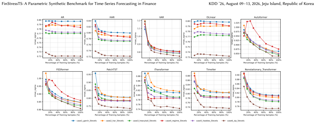
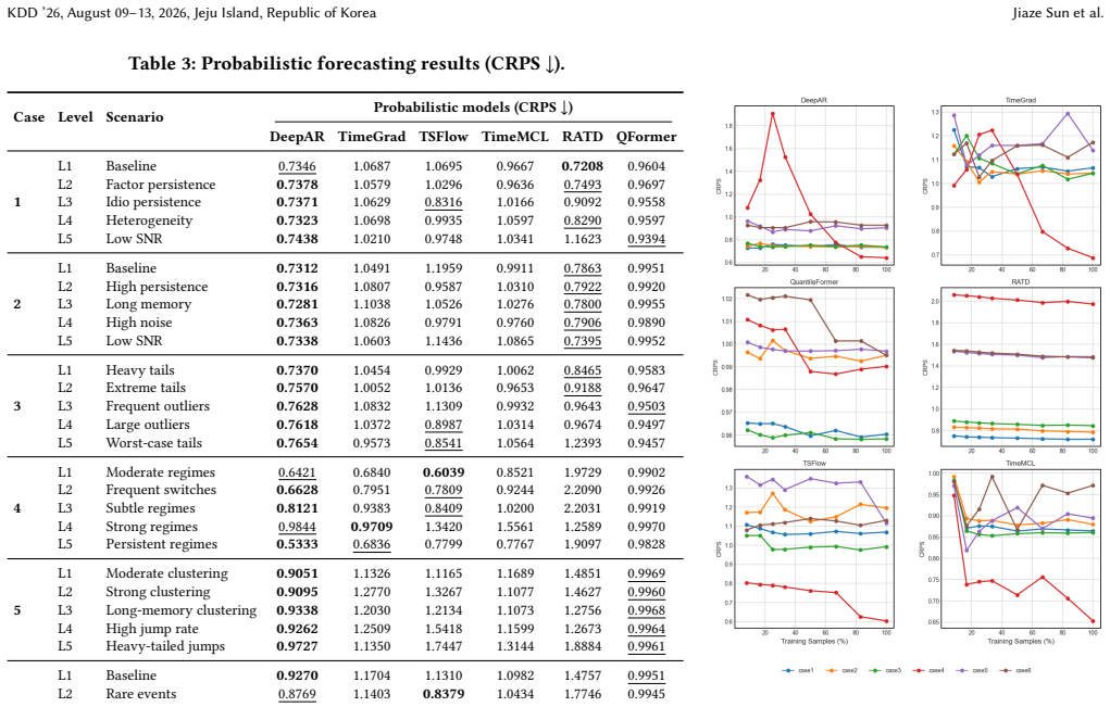
FinStressTS comprises thirty diagnostic environments around six mechanism families—volatility clustering, multi-scale persistence, heavy-tailed shocks, regime switching, self-exciting jumps, and zero-inflated processes—and shows that autoregressive and linear models remain competitive or superior in several volatility-, tail-, and jump-driven settings while parametric probabilistic models calibrate well in stationary regimes.
What carries the argument
The six parametric mechanism families that generate the thirty diagnostic environments, each isolating one structural cause so that model errors can be attributed to a known data-generating process.
If this is right
- Autoregressive and linear models are highly competitive in volatility-, tail-, and jump-driven environments.
- Parametric probabilistic models such as DeepAR calibrate well in stationary settings, while flexible models help when distributions become multimodal or sparse.
- Neural models often require more data to match simple baselines, with larger gains mainly when learning latent regimes or complex distributions.
Where Pith is reading between the lines
- Model selection pipelines in finance could become conditional on detected mechanism type rather than fixed across all assets.
- The same parametric construction could be reused to generate stress-test suites for regulatory capital calculations under known tail and jump scenarios.
- Learning curves measured on these environments offer a direct way to quantify how much additional data a new architecture needs before it surpasses a linear baseline.
Load-bearing premise
The six parametric mechanism families accurately reproduce the latent structural causes present in real financial time series without adding correlations or artifacts absent from actual markets.
What would settle it
If the relative performance ordering of the fifteen models on real financial series differs systematically from their ordering on the matching FinStressTS environments, the claim that the benchmark isolates the relevant mechanisms would be undermined.
Figures

read the original abstract
Financial forecasting is difficult due to low signal-to-noise ratios, latent factors, heavy tails, regime shifts, and jumps. Real-world benchmarks offer limited failure attribution: researchers can observe underperformance, but often cannot isolate why because mechanisms are unobservable and entangled. Real financial data reveal only one realized path, making it difficult to assess tail-risk calibration or data efficiency. We introduce FinStressTS, a mechanism-aware synthetic benchmark that links model behavior to controlled structural causes. FinStressTS comprises 30 diagnostic environments around six mechanism families: volatility clustering, multi-scale persistence, heavy-tailed shocks, regime switching, self-exciting jumps, and zero-inflated processes. We evaluate two tasks: point forecasting, using NMAE across five settings, and probabilistic forecasting, using CRPS under known data-generating mechanisms. We benchmark 15 models, from classical methods (HAR, VAR) to Transformer forecasters (PatchTST, iTransformer) and deep probabilistic architectures (DeepAR, TSFlow), and use learning curves to measure sample efficiency. Our evaluation reveals three insights. First, performance is mechanism-dependent: autoregressive and linear models are highly competitive, and often outperform Transformer-based models, in several volatility-, tail-, and jump-driven environments. Second, distributional alignment matters: parametric probabilistic models such as DeepAR calibrate well in stationary settings, while flexible models can help when distributions become multimodal or sparse. Third, neural models often require more data to match simple baselines, with larger gains mainly when learning latent regimes or complex distributions. FinStressTS provides an open framework for diagnosing failure modes and advancing risk-aware forecasting.
Editorial analysis
A structured set of objections, weighed in public.
Referee Report
Summary. The paper introduces FinStressTS, a synthetic benchmark with 30 diagnostic environments built from six parametric mechanism families (volatility clustering, multi-scale persistence, heavy-tailed shocks, regime switching, self-exciting jumps, zero-inflated processes). It evaluates 15 models (HAR, VAR, PatchTST, iTransformer, DeepAR, TSFlow, etc.) on point forecasting via NMAE and probabilistic forecasting via CRPS under known DGPs, plus learning curves for sample efficiency, and reports three insights: mechanism-dependent performance (AR/linear models competitive in volatility/tail/jump settings), importance of distributional alignment for calibration, and higher data needs for neural models except in regime/complex-distribution cases.
Significance. If the environments isolate the claimed mechanisms, the benchmark supplies a controlled testbed that real financial series cannot, because the latter entangle latent factors and provide only one path. This would allow precise attribution of failure modes (e.g., poor tail calibration under jumps versus regime shifts) and targeted model improvement for risk-aware forecasting. The open framework and broad model coverage constitute a useful public resource for the field.
major comments (1)
- [six parametric mechanism families and 30 diagnostic environments] The claim that 'performance is mechanism-dependent' (abstract) and the three insights require that each of the six families operates in isolation within its 30 environments. Self-exciting jumps (Hawkes-type) generate clustered large increments that automatically raise the autocorrelation of squared returns, thereby injecting an unintended volatility-clustering signature into a 'jumps-only' environment. Regime-switching constructions can similarly induce spurious persistence or heavy tails. The manuscript must supply explicit orthogonality diagnostics (e.g., moment or spectral comparisons across families) to confirm the diagnostic mapping is valid; absent such checks the attribution of model rankings to specific structural causes is compromised.
minor comments (1)
- [abstract] The abstract states the benchmark design and high-level results but supplies no equations, parameter values, or validation statistics; readers must consult the full text for reproducibility details.
Simulated Author's Rebuttal
We thank the referee for highlighting the critical need to verify isolation of the six mechanism families. We agree that potential cross-contamination (e.g., Hawkes-induced volatility clustering) could weaken attribution of the reported insights, and we will strengthen the manuscript with the requested diagnostics.
read point-by-point responses
-
Referee: [six parametric mechanism families and 30 diagnostic environments] The claim that 'performance is mechanism-dependent' (abstract) and the three insights require that each of the six families operates in isolation within its 30 environments. Self-exciting jumps (Hawkes-type) generate clustered large increments that automatically raise the autocorrelation of squared returns, thereby injecting an unintended volatility-clustering signature into a 'jumps-only' environment. Regime-switching constructions can similarly induce spurious persistence or heavy tails. The manuscript must supply explicit orthogonality diagnostics (e.g., moment or spectral comparisons across families) to confirm the diagnostic mapping is valid; absent such checks the attribution of model rankings to specific structural causes is compromised.
Authors: We agree that the validity of mechanism-dependent performance claims rests on demonstrating that each family primarily isolates its intended structure. While the parametric constructions were chosen to emphasize one dominant feature per family (e.g., Hawkes intensity for jumps, Markov switching for regimes), we acknowledge that secondary signatures such as elevated squared-return autocorrelation in jump environments or induced kurtosis in regime environments may exist. In the revision we will add a new subsection (Section 3.3) containing explicit orthogonality checks: (i) autocorrelation functions of raw and squared series, (ii) kurtosis and tail-index estimates, and (iii) spectral density comparisons across all 30 environments. These diagnostics will quantify the degree of unintended overlap and, where necessary, adjust environment parameters to improve isolation. The three insights will be re-stated with reference to these checks. revision: yes
Circularity Check
No circularity: benchmark generation and empirical evaluation are independent of fitted results
full rationale
The paper constructs FinStressTS by specifying six parametric mechanism families (volatility clustering, regime switching, etc.) and 30 diagnostic environments, then runs standard point and probabilistic forecasting metrics (NMAE, CRPS) plus learning curves on 15 models. No equation or claim reduces a reported performance insight to a quantity defined by parameters fitted inside the same paper; the data-generating processes are fixed by construction before any model is applied, and the reported mechanism-dependent rankings are direct outputs of those evaluations rather than self-referential fits. No self-citation chain is invoked to justify uniqueness or an ansatz, and no known empirical pattern is merely renamed.
Axiom & Free-Parameter Ledger
Reference graph
Works this paper leans on
-
[1]
Alexander Alexandrov, Konstantinos Benidis, Michael Bohlke-Schneider, Valentin Flunkert, Jan Gasthaus, Tim Januschowski, Danielle C Maddix, Syama Rangapu- ram, David Salinas, Jasper Schulz, et al. 2020. Gluonts: Probabilistic and neural time series modeling in python.Journal of Machine Learning Research21, 116 (2020), 1–6
2020
-
[2]
Torben G Andersen, Tim Bollerslev, and Francis X Diebold. 2007. Roughing it up: Including jump components in the measurement, modeling, and forecasting of return volatility.The review of economics and statistics89, 4 (2007), 701–720
2007
-
[3]
Torben G Andersen, Tim Bollerslev, Francis X Diebold, and Paul Labys. 2003. Modeling and forecasting realized volatility.Econometrica71, 2 (2003), 579–625
2003
-
[4]
Andersen, Tim Bollerslev, Francis X
Torben G. Andersen, Tim Bollerslev, Francis X. Diebold, and Paul Labys. 2003. Modeling and Forecasting Realized Volatility.Econometrica71, 2 (2003), 579–625. doi:10.1111/1468-0262.00402
-
[5]
Yihao Ang, Qiang Huang, Yifan Bao, Anthony KH Tung, and Zhiyong Huang
-
[6]
TSGBench: Time Series Generation Benchmark.Proceedings of the VLDB Endowment17, 3 (2023), 305–318
2023
-
[7]
Emmanuel Bacry, Iacopo Mastromatteo, and Jean-François Muzy. 2015. Hawkes Processes in Finance.Market Microstructure and Liquidity1, 1 (2015), 1550005. doi:10.1142/S2382626615500057
-
[8]
Tim Bollerslev. 1986. Generalized Autoregressive Conditional Heteroskedasticity. Journal of Econometrics31, 3 (1986), 307–327. doi:10.1016/0304-4076(86)90063-1
-
[9]
Tim Bollerslev. 1987. A Conditionally Heteroskedastic Time Series Model for Speculative Prices and Rates of Return.The Review of Economics and Statistics69, 3 (1987), 542–547
1987
-
[10]
George Box and GM Jenkins. 1976. Analysis: Forecasting and Control.San francisco(1976)
1976
-
[11]
Weijun Chen, Shun Li, Xipu Yu, Heyuan Wang, Wei Chen, and Tengjiao Wang
-
[12]
InProceedings of the Thirty-Third International Joint Conference on Artificial Intelligence
Automatic de-biased temporal-relational modeling for stock investment recommendation. InProceedings of the Thirty-Third International Joint Conference on Artificial Intelligence. 1999–2008
1999
-
[13]
Rama Cont. 2001. Empirical properties of asset returns: stylized facts and statisti- cal issues.Quantitative Finance1, 2 (2001), 223–236. doi:10.1080/713665670
-
[14]
Rama Cont. 2001. Empirical properties of asset returns: stylized facts and statisti- cal issues.Quantitative finance1, 2 (2001), 223. KDD ’26, August 09–13, 2026, Jeju Island, Republic of Korea Jiaze Sun et al
2001
-
[15]
Fulvio Corsi. 2009. A Simple Approximate Long-Memory Model of Realized Volatility.Journal of Financial Econometrics7, 2 (2009), 174–196. doi:10.1093/ jjfinec/nbp001
2009
-
[16]
Fulvio Corsi. 2009. A simple approximate long-memory model of realized volatil- ity.Journal of financial econometrics7, 2 (2009), 174–196
2009
-
[17]
Adrien Cortés, Rémi Rehm, and Victor Letzelter. 2025. Winner-takes-all for Multi- variate Probabilistic Time Series Forecasting. InICML 2025: The 42nd International Conference on Machine Learning
2025
-
[18]
Yitong Duan, Lei Wang, Qizhong Zhang, and Jian Li. 2022. Factorvae: A proba- bilistic dynamic factor model based on variational autoencoder for predicting cross-sectional stock returns. InProceedings of the AAAI conference on artificial intelligence, Vol. 36. 4468–4476
2022
-
[19]
Straßburger (2013): Cut Elimination in Nested Sequents for Intuitionistic Modal Logics
Paul Embrechts, Claudia Klüppelberg, and Thomas Mikosch. 1997.Modelling Extremal Events for Insurance and Finance. Springer. doi:10.1007/978-3-642- 33483-2
-
[20]
Robert F Engle. 1982. Autoregressive conditional heteroscedasticity with esti- mates of the variance of United Kingdom inflation.Econometrica: Journal of the econometric society(1982), 987–1007
1982
-
[21]
Robert F. Engle. 1982. Autoregressive Conditional Heteroskedasticity with Esti- mates of the Variance of United Kingdom Inflation.Econometrica50, 4 (1982), 987–1007. doi:10.2307/1912773
-
[22]
Eugene F Fama and Kenneth R French. 1993. Common risk factors in the returns on stocks and bonds.Journal of financial economics33, 1 (1993), 3–56
1993
-
[23]
Muhammad Hasan Ferdous, Emam Hossain, and Md Osman Gani. 2025. Time- graph: Synthetic benchmark datasets for robust time-series causal discovery. In Proceedings of the 31st ACM SIGKDD Conference on Knowledge Discovery and Data Mining V. 2. 5425–5435
2025
-
[24]
Tilmann Gneiting and Matthias Katzfuss. 2014. Probabilistic forecasting.Annual Review of Statistics and Its Application1, 1 (2014), 125–151
2014
-
[25]
Tilmann Gneiting and Adrian E. Raftery. 2007. Strictly Proper Scoring Rules, Prediction, and Estimation.J. Amer. Statist. Assoc.102, 477 (2007), 359–378. doi:10.1198/016214506000001437
- [26]
-
[27]
James D Hamilton. 1989. A new approach to the economic analysis of nonstation- ary time series and the business cycle.Econometrica: Journal of the econometric society(1989), 357–384
1989
-
[28]
Alan G. Hawkes. 1971. Spectra of some self-exciting and mutually exciting point processes.Biometrika58, 1 (1971), 83–90. doi:10.1093/biomet/58.1.83
-
[29]
Yifan Hu, Yuante Li, Peiyuan Liu, Yuxia Zhu, Naiqi Li, Tao Dai, Shu-tao Xia, Dawei Cheng, and Changjun Jiang. 2025. Fintsb: A comprehensive and practical benchmark for financial time series forecasting.arXiv preprint arXiv:2502.18834 (2025)
work page internal anchor Pith review Pith/arXiv arXiv 2025
-
[30]
Yanfei Kang, Rob J Hyndman, and Feng Li. 2020. GRATIS: GeneRAting TIme Series with diverse and controllable characteristics.Statistical Analysis and Data Mining: The ASA Data Science Journal13, 4 (2020), 354–376
2020
- [31]
-
[32]
Diane Lambert. 1992. Zero-Inflated Poisson Regression, with an Application to Defects in Manufacturing.Technometrics34, 1 (1992), 1–14. doi:10.1080/00401706. 1992.10485228
-
[33]
David A. Lesmond, Joseph P. Ogden, and Charles A. Trzcinka. 1999. A New Estimate of Transaction Costs.The Review of Financial Studies12, 5 (1999), 1113–1141. doi:10.1093/rfs/12.5.1113
-
[34]
Jingwei Liu, Ling Yang, Hongyan Li, and Shenda Hong. 2024. Retrieval-augmented diffusion models for time series forecasting.Advances in Neural Information Processing Systems37 (2024), 2766–2786
2024
-
[35]
Yong Liu, Tengge Hu, Haoran Zhang, Haixu Wu, Shiyu Wang, Lintao Ma, and Mingsheng Long. 2023. itransformer: Inverted transformers are effective for time series forecasting.arXiv preprint arXiv:2310.06625(2023)
work page internal anchor Pith review Pith/arXiv arXiv 2023
-
[36]
Yong Liu, Haixu Wu, Jianmin Wang, and Mingsheng Long. 2022. Non-stationary transformers: Exploring the stationarity in time series forecasting.Advances in neural information processing systems35 (2022), 9881–9893
2022
- [37]
-
[38]
2013.Introduction to multiple time series analysis
Helmut Lütkepohl. 2013.Introduction to multiple time series analysis. Springer Science & Business Media
2013
-
[39]
Spyros Makridakis and Michele Hibon. 2000. The M3-Competition: results, conclusions and implications.International journal of forecasting16, 4 (2000), 451–476
2000
-
[40]
Spyros Makridakis, Evangelos Spiliotis, and Vassilios Assimakopoulos. 2018. The M4 Competition: Results, findings, conclusion and way forward.International Journal of forecasting34, 4 (2018), 802–808
2018
-
[41]
Spyros Makridakis, Evangelos Spiliotis, Ross Hollyman, Fotios Petropoulos, Nor- man Swanson, and Anil Gaba. 2024. The M6 forecasting competition: Bridging the gap between forecasting and investment decisions.International Journal of Forecasting(2024)
2024
-
[42]
James E Matheson and Robert L Winkler. 1976. Scoring rules for continuous probability distributions.Management science22, 10 (1976), 1087–1096
1976
-
[43]
Y Nie. 2022. A Time Series is Worth 64Words: Long-term Forecasting with Transformers.arXiv preprint arXiv:2211.14730(2022)
work page internal anchor Pith review Pith/arXiv arXiv 2022
-
[44]
Alexander Nikitin, Letizia Iannucci, and Samuel Kaski. 2024. TSGM: a flexible framework for generative modeling of synthetic time series.Advances in Neural Information Processing Systems37 (2024), 129042–129061
2024
-
[45]
Olivares, Cristian Challú, Azul Garza, Max Mergenthaler Canseco, and Artur Dubrawski
Kin G. Olivares, Cristian Challú, Azul Garza, Max Mergenthaler Canseco, and Artur Dubrawski. 2022. NeuralForecast: User friendly state-of-the-art neural forecasting models. PyCon Salt Lake City, Utah, US 2022. https://github.com/ Nixtla/neuralforecast
2022
-
[46]
Cemal Öztürk. 2024. Enhancing Financial Time-Series Analysis with TimeGAN: A Novel Approach. In2024 9th International Conference on Computer Science and Engineering (UBMK). IEEE, 447–450
2024
-
[47]
Xiangfei Qiu, Jilin Hu, Lekui Zhou, Xingjian Wu, Junyang Du, Buang Zhang, Chenjuan Guo, Aoying Zhou, Christian S Jensen, Zhenli Sheng, et al. 2024. TFB: Towards Comprehensive and Fair Benchmarking of Time Series Forecasting Methods.Proceedings of the VLDB Endowment17, 9 (2024), 2363–2377
2024
-
[48]
Kashif Rasul, Calvin Seward, Ingmar Schuster, and Roland Vollgraf. 2021. Au- toregressive denoising diffusion models for multivariate probabilistic time series forecasting. InInternational conference on machine learning. PMLR, 8857–8868
2021
-
[49]
Stephen A Ross. 2013. The arbitrage theory of capital asset pricing. InHandbook of the fundamentals of financial decision making: Part I. World Scientific, 11–30
2013
-
[50]
David Salinas, Valentin Flunkert, Jan Gasthaus, and Tim Januschowski. 2020. DeepAR: Probabilistic forecasting with autoregressive recurrent networks.Inter- national journal of forecasting36, 3 (2020), 1181–1191
2020
-
[51]
Yimiao Shao, Wenzhong Li, Kang Xia, Kaijie Lin, Mingkai Lin, and Sanglu Lu. 2025. QuantileFormer: Probabilistic Time Series Forecasting with a Pattern-Mixture Decomposed VAE Transformer. InProceedings of the Thirty-Fourth International Joint Conference on Artificial Intelligence. 6147–6155
2025
-
[52]
Zezhi Shao, Fei Wang, Yongjun Xu, Wei Wei, Chengqing Yu, Zhao Zhang, Di Yao, Tao Sun, Guangyin Jin, Xin Cao, et al. 2024. Exploring progress in multi- variate time series forecasting: Comprehensive benchmarking and heterogeneity analysis.IEEE Transactions on Knowledge and Data Engineering37, 1 (2024), 291–305
2024
-
[53]
Sean J Taylor and Benjamin Letham. 2018. Forecasting at scale.The American Statistician72, 1 (2018), 37–45
2018
-
[54]
Heyuan Wang, Tengjiao Wang, Shun Li, Jiayi Zheng, Shijie Guan, and Wei Chen
-
[55]
Adaptive Long-Short Pattern Transformer for Stock Investment Selection.. InIJCAI. 3970–3977
-
[56]
Yuxuan Wang, Haixu Wu, Jiaxiang Dong, Yong Liu, Mingsheng Long, and Jianmin Wang. 2024. Deep Time Series Models: A Comprehensive Survey and Benchmark. (2024)
2024
-
[57]
Yuxuan Wang, Haixu Wu, Jiaxiang Dong, Guo Qin, Haoran Zhang, Yong Liu, Yunzhong Qiu, Jianmin Wang, and Mingsheng Long. 2024. Timexer: Empowering transformers for time series forecasting with exogenous variables.Advances in Neural Information Processing Systems37 (2024), 469–498
2024
-
[58]
Magnus Wiese, Robert Knobloch, Ralf Korn, and Peter Kretschmer. 2020. Quant GANs: deep generation of financial time series.Quantitative Finance20, 9 (2020), 1419–1440
2020
-
[59]
Haixu Wu, Jiehui Xu, Jianmin Wang, and Mingsheng Long. 2021. Autoformer: De- composition transformers with auto-correlation for long-term series forecasting. Advances in neural information processing systems34 (2021), 22419–22430
2021
-
[60]
Ailing Zeng, Muxi Chen, Lei Zhang, and Qiang Xu. 2023. Are transformers effective for time series forecasting?. InProceedings of the AAAI conference on artificial intelligence, Vol. 37. 11121–11128
2023
-
[61]
Liang Zeng, Lei Wang, Hui Niu, Ruchen Zhang, Ling Wang, and Jian Li. 2024. Trade when opportunity comes: price movement forecasting via locality-aware attention and iterative refinement labeling. InProceedings of the Thirty-Third International Joint Conference on Artificial Intelligence. 6134–6142
2024
-
[62]
Jiawen Zhang, Xumeng Wen, Zhenwei Zhang, Shun Zheng, Jia Li, and Jiang Bian
-
[63]
ProbTS: Benchmarking point and distributional forecasting across diverse prediction horizons.Advances in Neural Information Processing Systems37 (2024), 48045–48082
2024
-
[64]
Tian Zhou, Ziqing Ma, Qingsong Wen, Xue Wang, Liang Sun, and Rong Jin. 2022. Fedformer: Frequency enhanced decomposed transformer for long-term series forecasting. InInternational conference on machine learning. PMLR, 27268–27286. FinStressTS: A Parametric Synthetic Benchmark for Time-Series Forecasting in Finance KDD ’26, August 09–13, 2026, Jeju Island,...
2022
discussion (0)
Sign in with ORCID, Apple, or X to comment. Anyone can read and Pith papers without signing in.