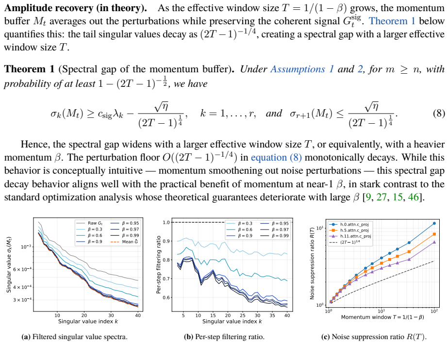
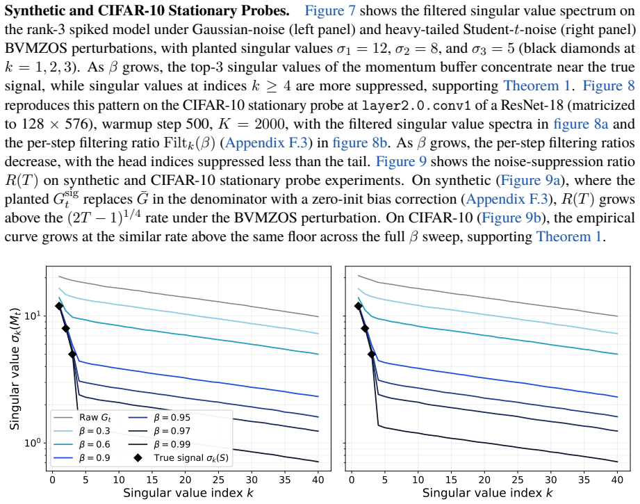
Denoise First, Orthogonalize Later: Understanding Momentum in Muon via Spectral Filtering
Pith reviewed 2026-06-28 11:22 UTC · model grok-4.3
The pith
Momentum in Muon acts as a spectral filter that enlarges the gap between signal and perturbations before orthogonalization.
A machine-rendered reading of the paper's core claim, the machinery that carries it, and where it could break.
Core claim
Under a structured signal-plus-perturbation gradient model, momentum suppresses perturbations while preserving the dominant signal, thereby enlarging the spectral gap between them. This enlarged gap stabilizes the singular subspaces of the matrix passed to Muon's orthogonalization step, making the resulting update more reliable. We further show that applying momentum before orthogonalization achieves provably stronger alignment with the signal component of the gradient than either reversing this order or simply removing momentum.
What carries the argument
Momentum as a spectral filter that enlarges the gap between dominant signal and perturbations in the gradient matrix before the orthogonalization step.
If this is right
- Momentum before orthogonalization yields stronger alignment with the signal component of the gradient.
- The orthogonalized update becomes more reliable due to stabilized singular subspaces.
- This mechanism explains observed performance gains in Muon with momentum.
- The theory extends to other matrix-based optimizers using similar steps.
Where Pith is reading between the lines
- Similar filtering benefits might appear in other optimizers that combine momentum with matrix decompositions.
- The signal-plus-perturbation model could be used to derive optimal momentum coefficients for specific gradient structures.
- Testing on gradients without clear spectral gaps would clarify the model's applicability.
Load-bearing premise
The gradient follows a structured signal-plus-perturbation model in which momentum enlarges the spectral gap.
What would settle it
Measure the singular subspace alignment or update reliability in a setting where the gradient lacks a clear dominant signal component separated from perturbations and check whether momentum still improves performance.
Figures


read the original abstract
Muon has recently demonstrated strong empirical performance in large language model training, but the theoretical role of momentum in Muon remains unclear. Existing analyses of Muon either remove momentum to study spectral updates in isolation, or retain momentum without explaining why it improves empirical performance. Our work bridges this gap by showing momentum in Muon acts as a spectral filter. Under a structured signal-plus-perturbation gradient model, we prove that momentum suppresses perturbations while preserving the dominant signal, thereby enlarging the spectral gap between them. This enlarged gap stabilizes the singular subspaces of the matrix passed to Muon's orthogonalization step, making the resulting update more reliable. We further show that applying momentum before orthogonalization achieves provably stronger alignment with the signal component of the gradient than either reversing this order or simply removing momentum. Experiments across diverse tasks, including LLM pretraining, support our theoretical analysis. More broadly, our theory offers a starting point for understanding the benefits of momentum in other matrix-based optimizers.
Editorial analysis
A structured set of objections, weighed in public.
Referee Report
Summary. The paper claims that under an explicitly stated structured signal-plus-perturbation model for gradients, momentum in Muon functions as a spectral low-pass filter: it suppresses perturbation components while preserving the dominant signal, thereby enlarging the gap between their singular values. This gap enlargement is shown to stabilize the singular subspaces passed to Muon's orthogonalization step (via Davis-Kahan-type bounds), and applying momentum before orthogonalization is proved to yield stronger signal alignment than the reverse order or momentum-free updates. Experiments on diverse tasks including LLM pretraining are reported as supporting evidence.
Significance. If the gradient model is realistic, the work supplies a conditional but rigorous theoretical account of momentum's benefit in Muon, filling a gap left by prior analyses that either omit momentum or retain it without explanation. The explicit model definition, direct derivation of the filtering effect and ordering claim, and supporting experiments constitute clear strengths; the analysis is internally consistent on its stated terms. The potential circularity concern raised in the stress-test note does not land, as the model is presented as the scope of the proof rather than a hidden premise tuned post hoc.
minor comments (2)
- [Abstract] Abstract, final sentence: the phrase 'starting point for understanding the benefits of momentum in other matrix-based optimizers' would benefit from a brief forward reference to the discussion section where this extension is sketched.
- [§4] §4 (Experiments): Table 1 caption could explicitly note the number of random seeds used for the reported means and standard deviations to improve clarity of statistical reliability.
Simulated Author's Rebuttal
We thank the referee for their positive assessment of the manuscript and for recommending acceptance. The referee's summary accurately reflects the paper's claims, model assumptions, and experimental support. No major comments were raised that require point-by-point rebuttal.
Circularity Check
No significant circularity: conditional proof under explicit model
full rationale
The central derivation is a conditional proof that momentum enlarges the spectral gap under an explicitly stated signal-plus-perturbation gradient model, followed by standard Davis-Kahan subspace perturbation bounds. The model is introduced as an assumption defining the scope of the analysis rather than being fitted to data or defined in terms of the desired filtering outcome. No load-bearing steps reduce to self-citation chains, fitted parameters renamed as predictions, or ansatzes smuggled via prior work. Experiments on LLM pretraining supply independent empirical checks outside the model. The argument is therefore self-contained on its stated terms and does not collapse to its inputs by construction.
Axiom & Free-Parameter Ledger
axioms (1)
- domain assumption Gradient admits a structured decomposition into dominant signal plus perturbation such that momentum enlarges their spectral gap
Reference graph
Works this paper leans on
-
[1]
Amsel, D
N. Amsel, D. Persson, C. Musco, and R. M. Gower. The polar express: Optimal matrix sign methods and their application to the Muon algorithm. InProceedings of the 14th International Conference on Learning Representations, 2026. (cited on p. 18)
2026
-
[2]
J. Ba, M. A. Erdogdu, T. Suzuki, Z. Wang, D. Wu, and G. Yang. High-dimensional asymptotics of featurelearning: Howonegradientstepimprovestherepresentation.AdvancesinNeuralInformation Processing Systems, 35:37932–37946, 2022. (cited on pp. 4 and 19)
2022
-
[3]
J. Bochnak, M. Coste, and M.-F. Roy.Real Algebraic Geometry, volume 36 ofErgebnisse der Mathematik und ihrer Grenzgebiete. 3. Folge / A Series of Modern Surveys in Mathematics. Springer- Verlag, Berlin, 1998. doi: 10.1007/978-3-662-03718-8. (cited on p. 24)
-
[4]
Boreiko, Z
V. Boreiko, Z. Bu, and S. Zha. Towards understanding orthogonalization in Muon. InProceedings of the 3rd Workshop on Efficient Systems for Foundation Models, 2025. (cited on p. 18)
2025
-
[5]
G.Braun,H.Bao,W.Huang,andM.Imaizumi. Spectralgradientdescentmitigatesanisotropy-driven misalignment: A case study in phase retrieval.arXiv preprint arXiv:2601.22652, 2026. (cited on pp. 4 and 18). 12
-
[6]
Busbridge, J
D. Busbridge, J. Ramapuram, P. Ablin, T. Likhomanenko, E. G. Dhekane, X. Suau Cuadros, and R. Webb. How to scale your EMA.Advances in Neural Information Processing Systems, 36: 73122–73174, 2023. (cited on p. 19)
2023
-
[7]
Carlson, V
D. Carlson, V. Cevher, and L. Carin. Stochastic spectral descent for restricted Boltzmann machines. InProceedings of the 18th International Conference on Artificial Intelligence and Statistics, pages 111–119. PMLR, 2015. (cited on p. 18)
2015
-
[8]
Carlson, E
D. Carlson, E. Collins, Y.-P. Hsieh, L. Carin, and V. Cevher. Preconditioned spectral descent for deep learning.Advances in Neural Information Processing Systems, 28:2971–2979, 2015. (cited on p. 18)
2015
-
[9]
Muonoptimizesunderspectralnormconstraints.TransactionsonMachine Learning Research, 2026
L.Chen,J.Li,andQ.Liu. Muonoptimizesunderspectralnormconstraints.TransactionsonMachine Learning Research, 2026. (cited on pp. 2, 6, and 18)
2026
-
[10]
Chikuse.Statistics on Special Manifolds, volume 174
Y. Chikuse.Statistics on Special Manifolds, volume 174. Springer Science & Business Media, 2003. (cited on p. 27)
2003
-
[11]
Cutkosky and H
A. Cutkosky and H. Mehta. Momentum improves normalized SGD. InProceedings of the 37th International Conference on Machine Learning, pages 2260–2268. PMLR, 2020. (cited on pp. 1 and 18)
2020
-
[12]
arXiv preprint arXiv:2512.04299 , year=
D. Davis and D. Drusvyatskiy. When do spectral gradient updates help in deep learning?arXiv preprint arXiv:2512.04299, 2025. (cited on pp. 2 and 18)
- [13]
-
[14]
RMNP: Row-Momentum Normalized Preconditioning for Scalable Matrix-Based Optimization
S.Deng,Z.Ouyang,T.Pang,Z.Liu,R.Jin,S.Yu,andY.Yang. RMNP:Row-momentumnormalized preconditioning for scalable matrix-based optimization.arXiv preprint arXiv:2603.20527, 2026. (cited on p. 18)
work page internal anchor Pith review Pith/arXiv arXiv 2026
-
[15]
C. Fan, M. Schmidt, and C. Thrampoulidis. Implicit bias of spectral descent and Muon on multiclass separable data.Advances in Neural Information Processing Systems, 38:39622–39669, 2025. (cited on pp. 2, 6, and 18)
2025
-
[16]
E. S. Gardner Jr. Exponential smoothing: The state of the art.Journal of Forecasting, 4(1):1–28,
-
[17]
4 and 19)
(cited on pp. 4 and 19)
-
[18]
Ghorbani, S
B. Ghorbani, S. Krishnan, and Y. Xiao. An investigation into neural net optimization via Hessian eigenvaluedensity. InProceedingsofthe36thInternationalConferenceonMachineLearning,pages 2232–2241. PMLR, 2019. (cited on p. 19)
2019
-
[19]
Ghosh, D
N. Ghosh, D. Wu, and A. Bietti. Understanding the mechanisms of fast hyperparameter transfer. InProceedings of the 14th International Conference on Learning Representations, 2026. (cited on p. 4)
2026
-
[20]
G. Goh. Why momentum really works.Distill, 2017. doi: 10.23915/distill.00006. (cited on p. 18)
-
[21]
Gupta, T
V. Gupta, T. Koren, and Y. Singer. Shampoo: Preconditioned stochastic tensor optimization. In Proceedings of the 35th International Conference on Machine Learning, pages 1842–1850. PMLR,
-
[22]
1 and 18)
(cited on pp. 1 and 18)
-
[23]
Gradient Descent Happens in a Tiny Subspace
G. Gur-Ari, D. A. Roberts, and E. Dyer. Gradient descent happens in a tiny subspace.arXiv preprint arXiv:1812.04754, 2018. (cited on pp. 4 and 19). 13
work page internal anchor Pith review Pith/arXiv arXiv 2018
-
[24]
C. He, Z. Deng, and Z. Lu. Low-rank orthogonalization for large-scale matrix optimization with applications to foundation model training.arXiv preprint arXiv:2509.11983, 2025. (cited on p. 18)
work page internal anchor Pith review Pith/arXiv arXiv 2025
-
[25]
N. J. Higham.Functions of Matrices: Theory and Computation. SIAM, 2008. (cited on p. 28)
2008
-
[26]
Muon: Anoptimizerfor hiddenlayersinneuralnetworks,2024
K.Jordan,Y.Jin,V.Boza,J.You,F.Cesista,L.Newhouse,andJ.Bernstein. Muon: Anoptimizerfor hiddenlayersinneuralnetworks,2024. URL https://kellerjordan.github.io/posts/muon/. (cited on pp. 1, 2, 3, and 18)
2024
-
[27]
J. Kim, E. Nichani, D. Wu, A. Bietti, and J. D. Lee. Sharp capacity scaling of spectral optimizers in learning associative memory.arXiv preprint arXiv:2603.26554, 2026. (cited on pp. 2 and 18)
work page internal anchor Pith review Pith/arXiv arXiv 2026
-
[28]
D. P. Kingma and J. Ba. Adam: A method for stochastic optimization. InProceedings of the 3rd International Conference on Learning Representations, 2015. (cited on p. 1)
2015
- [29]
-
[30]
B. Li, K. Wang, H. Zhong, P. Lu, and L. Wang. Muon in associative memory learning: Training dynamics and scaling laws.arXiv preprint arXiv:2602.05725, 2026. (cited on pp. 2 and 18)
work page internal anchor Pith review Pith/arXiv arXiv 2026
-
[31]
X. Li, J. Luo, Z. Zheng, H. Wang, L. Luo, L. Wen, L. Wu, and S. Xu. On the performance analysis of momentum method: A frequency domain perspective. InProceedings of the 13th International Conference on Learning Representations, 2025. (cited on pp. 2 and 18)
2025
-
[32]
J. Liu, J. Su, X. Yao, Z. Jiang, G. Lai, Y. Du, Y. Qin, W. Xu, E. Lu, J. Yan, Y. Chen, H. Zheng, Y. Liu, S. Liu, B. Yin, W. He, H. Zhu, Y. Wang, J. Wang, M. Dong, Z. Zhang, Y. Kang, H. Zhang, X. Xu, Y. Zhang, Y. Wu, X. Zhou, and Z. Yang. Muon is scalable for LLM training.arXiv preprint arXiv:2502.16982, 2025. (cited on pp. 1 and 18)
work page internal anchor Pith review Pith/arXiv arXiv 2025
-
[33]
W. Liu, R. Lin, Z. Liu, J. M. Rehg, L. Paull, L. Xiong, L. Song, and A. Weller. Orthogonal over- parameterizedtraining. In2021IEEE/CVFConferenceonComputerVisionandPatternRecognition, pages 7251–7260, 2021. (cited on p. 18)
2021
-
[34]
Loshchilov and F
I. Loshchilov and F. Hutter. Decoupled weight decay regularization. InProceedings of the 7th International Conference on Learning Representations, 2019. (cited on p. 1)
2019
- [35]
-
[36]
Mousavi-Hosseini, D
A. Mousavi-Hosseini, D. Wu, T. Suzuki, and M. A. Erdogdu. Gradient-based feature learning under structured data.Advances in Neural Information Processing Systems, 36:71449–71485, 2023. (cited on pp. 4 and 19)
2023
-
[37]
Nesterov
Y. Nesterov. A method for solving the convex programming problem with convergence rateo(1/k2). Soviet Mathematics Doklady, 27(2):372–376, 1983. (cited on pp. 1 and 18)
1983
-
[38]
Penedo, H
G. Penedo, H. Kydlíček, A. Lozhkov, M. Mitchell, C. Raffel, L. Von Werra, and T. Wolf. The FineWebdatasets: Decantingthewebforthefinesttextdataatscale.AdvancesinNeuralInformation Processing Systems, 37:30811–30849, 2024. (cited on p. 30)
2024
-
[39]
Pethick, W
T. Pethick, W. Xie, K. Antonakopoulos, Z. Zhu, A. Silveti-Falls, and V. Cevher. Training deep learning modelswithnorm-constrainedLMOs. InProceedingsofthe42ndInternationalConference on Machine Learning, pages 49069–49104, 2025. (cited on pp. 1 and 18). 14
2025
-
[40]
B. T. Polyak. Some methods of speeding up the convergence of iteration methods.USSR Computa- tional Mathematics and Mathematical Physics, 4(5):1–17, 1964. (cited on pp. 1 and 18)
1964
-
[41]
Z. Qiu, S. Buchholz, T. Z. Xiao, M. Dax, B. Schölkopf, and W. Liu. Reparameterized LLM training via orthogonal equivalence transformation.Advances in Neural Information Processing Systems, 38: 140775–140821, 2025. (cited on p. 18)
2025
-
[42]
Z. Qiu, L. Liu, A. Weller, H. Shi, and W. Liu. POET-X: Memory-efficient LLM training by scaling orthogonaltransformation.InProceedingsofthe43rdInternationalConferenceonMachineLearning. PMLR, 2026. (cited on p. 18)
2026
-
[43]
Raffel, N
C. Raffel, N. Shazeer, A. Roberts, K. Lee, S. Narang, M. Matena, Y. Zhou, W. Li, and P. J. Liu. Exploring the limits of transfer learning with a unified text-to-text transformer.Journal of Machine Learning Research, 21(140):1–67, 2020. (cited on p. 30)
2020
-
[44]
Riabinin, E
A. Riabinin, E. Shulgin, K. Gruntkowska, and P. Richtárik. Gluon: Making Muon & Scion great again! (bridging theory and practice of LMO-based optimizers for LLMs). InProceedings of the 3rd High-dimensional Learning Dynamics, 2025. (cited on p. 18)
2025
-
[45]
Empirical Analysis of the Hessian of Over-Parametrized Neural Networks
L. Sagun, U. Evci, V. U. Guney, Y. Dauphin, and L. Bottou. Empirical analysis of the Hessian of over-parametrized neural networks.arXiv preprint arXiv:1706.04454, 2017. (cited on p. 19)
work page internal anchor Pith review Pith/arXiv arXiv 2017
-
[46]
A. Semenov, M. Pagliardini, and M. Jaggi. Benchmarking optimizers for large language model pretraining.arXiv preprint arXiv:2509.01440, 2025. (cited on p. 1)
-
[47]
K. Shi, H. Li, Z. Qiu, Y. Wen, S. Buchholz, and W. Liu. Pion: A spectrum-preserving optimizer via orthogonal equivalence transformation.arXiv preprint arXiv:2605.12492, 2026. (cited on p. 18)
work page internal anchor Pith review Pith/arXiv arXiv 2026
-
[48]
Shulgin, S
E. Shulgin, S. AlRashed, P. Richtárik, and F. Orabona. Beyond the ideal: Analyzing the inexact Muon update. InProceedings of the 29th International Conference on Artificial Intelligence and Statistics, 2026. (cited on pp. 2, 6, and 18)
2026
-
[49]
Simsekli, L
U. Simsekli, L. Sagun, and M. Gurbuzbalaban. A tail-index analysis of stochastic gradient noise in deep neural networks. InProceedings of the 36th International Conference on Machine Learning, pages 5827–5837. PMLR, 2019. (cited on p. 19)
2019
-
[50]
Onthegeneralizationbenefitofnoiseinstochasticgradientdescent
S.Smith,E.Elsen,andS.De. Onthegeneralizationbenefitofnoiseinstochasticgradientdescent. In Proceedings of the 37th International Conference on Machine Learning, pages 9058–9067. PMLR,
-
[51]
J. Su, M. Ahmed, Y. Lu, S. Pan, W. Bo, and Y. Liu. RoFormer: Enhanced transformer with rotary position embedding.Neurocomputing, 568:127063, 2024. (cited on p. 37)
2024
- [52]
-
[53]
Sutskever, J
I. Sutskever, J. Martens, G. Dahl, and G. Hinton. On the importance of initialization and momentum in deep learning. InProceedings of the 30th International Conference on Machine Learning, pages 1139–1147. PMLR, 2013. (cited on pp. 1, 4, 18, and 19)
2013
-
[54]
LLaMA: Open and Efficient Foundation Language Models
H. Touvron, T. Lavril, G. Izacard, X. Martinet, M. Lachaux, T. Lacroix, B. Rozière, N. Goyal, E.Hambro,F.Azhar,A.Rodriguez,A.Joulin,E.Grave,andG.Lample. LLaMA:Openandefficient foundation language models.arXiv preprint arXiv:2302.13971, 2023. (cited on p. 30). 15
work page internal anchor Pith review Pith/arXiv arXiv 2023
-
[55]
M. Tuddenham, A. Prügel-Bennett, and J. Hare. Orthogonalising gradients to speed up neural network optimisation.arXiv preprint arXiv:2202.07052, 2022. (cited on pp. 2 and 18)
-
[56]
B. Vasudeva, P. Deora, Y. Zhao, V. Sharan, and C. Thrampoulidis. How Muon’s spectral design benefits generalization: A study on imbalanced data.arXiv preprint arXiv:2510.22980, 2025. (cited on p. 18)
-
[57]
Vershynin.High-dimensional Probability: An Introduction with Applications in Data Science, volume 47
R. Vershynin.High-dimensional Probability: An Introduction with Applications in Data Science, volume 47. Cambridge University Press, 2018. (cited on pp. 28 and 29)
2018
-
[58]
N. Vyas, D. Morwani, R. Zhao, I. Shapira, D. Brandfonbrener, L. Janson, and S. M. Kakade. SOAP: Improving and stabilizing Shampoo using Adam for language modeling. InProceedings of the 13th International Conference on Learning Representations, 2025. (cited on pp. 1 and 18)
2025
-
[59]
Themarginalvalueofmomentumforsmalllearning rate SGD
R.Wang,S.Malladi,T.Wang,K.Lyu,andZ.Li. Themarginalvalueofmomentumforsmalllearning rate SGD. InProceedings of the 12th International Conference on Learning Representations, 2024. (cited on p. 2)
2024
-
[60]
S.Wang,F.Zhang,J.Li,C.Du,C.Du,T.Pang,Z.Yang,M.Hong,andV.Y.Tan. Muonoutperforms Adam in tail-end associative memory learning.arXiv preprint arXiv:2509.26030, 2025. (cited on pp. 2 and 18)
-
[61]
P.-Å. Wedin. Perturbation bounds in connection with singular value decomposition.BIT Numerical Mathematics, 12(1):99–111, 1972. (cited on pp. 7 and 23)
1972
- [62]
-
[63]
Z. Zhu, J. Wu, B. Yu, L. Wu, and J. Ma. The anisotropic noise in stochastic gradient descent: Its behavior of escaping from sharp minima and regularization effects. InProceedings of the 36th International Conference on Machine Learning, pages 7654–7663. PMLR, 2019. (cited on p. 19). 16 Appendix Table of Contents A Related Work 18 B Setup Conventions and V...
2019
-
[64]
prove that momentum eliminates the large-batch requirement of normalized SGD, and Defazio[13] reformulates SGD with momentum as primal averaging to obtain sharper non-convex convergence bounds. Inspired by signal processing theory, Li et al.[29]interpret momentum in the frequency domain as a low- pass filter that amplifies low-frequency gradient component...
-
[65]
No weight is updated during gradient collection
Load the model from a saved checkpoint and hold every weight fixed, including the target weightW. No weight is updated during gradient collection
-
[66]
For t= 1, . . . , K , draw one mini-batch from the dataloader in its natural sequential order (the dataloader’s default ordering without shuffling), run one step of forward and backward propagation, and record the gradientGt of the target weightW. We refer to this as thesequentialcollection order, which is the default setting used throughout the paper. Fo...
-
[67]
The collection order is preserved because the downstream momentum buffers are order-dependent
Save the gradient sequence{Gt}K t=1 to disk in the order the mini-batches were drawn. The collection order is preserved because the downstream momentum buffers are order-dependent. Since the model weights do not change during gradient collection, everyGt is drawn from the same gradient distribution. This protocol therefore synthetically simulates the stat...
-
[68]
Each training step appendsGt to the buffer and pops the oldest entry once the buffer is full
Maintain a fixed-capacity First-In, First-Out (FIFO) buffer of the most recentK target weight’s gradients alongside the regular optimizer step. Each training step appendsGt to the buffer and pops the oldest entry once the buffer is full
-
[69]
, Gt}, run theAnalysis procedurebelow, and save the resulting summary
At everyI training step (we usedI= 100 in all CIFAR-10 and NanoGPT trajectory runs), take a checkpoint of the current buffer{Gt−K+1, . . . , Gt}, run theAnalysis procedurebelow, and save the resulting summary
-
[70]
The probe does not alter weight updates, optimizer state, random seeds, or data ordering
Continue training without modification. The probe does not alter weight updates, optimizer state, random seeds, or data ordering. The trajectory buffer therefore represents a sliding buffer over the live training trajectory, and the corre- sponding analysis quantities inherit any non-stationarity in the gradient stream. Buffer-size selection.The buffer si...
-
[71]
The top-r left and right singular vectors(Ur, Vr) define the signal subspace used as the alignment target on the CIFAR-10 and NanoGPT experiments
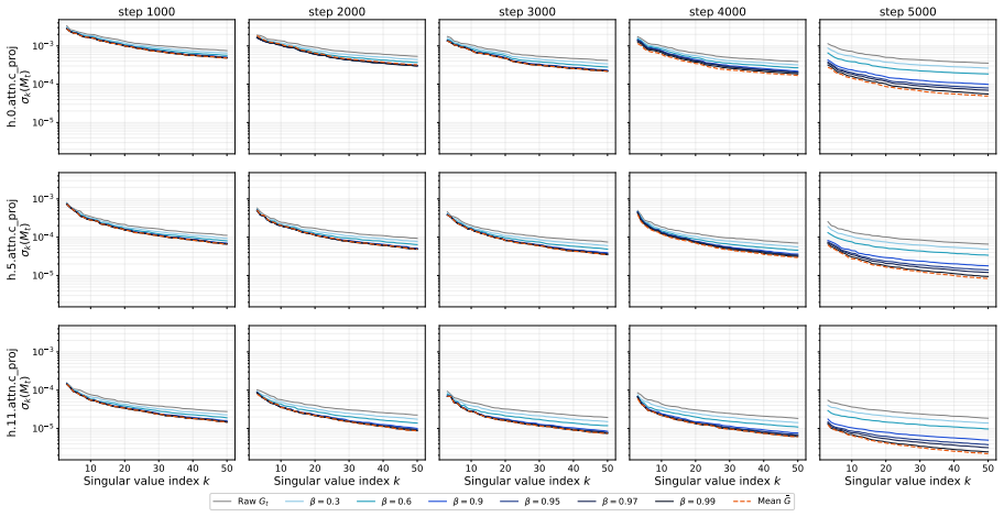
Signal reference.Compute the mean gradient¯G :=K −1PK t=1 Gt and its exact SVD¯G=UΣV ⊤. The top-r left and right singular vectors(Ur, Vr) define the signal subspace used as the alignment target on the CIFAR-10 and NanoGPT experiments. On the synthetic simulation the spiked model of Appendix F.4.1 plants a known rank-r⋆ signalG sig t with singular basesUtr...
-
[72]
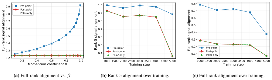
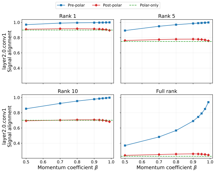
Threepipelines.Foreach β intheper-taskgrid(AppendixF.4),startingfrom M0 = fM0 = 0,Pre-polar 32 and Post-polar pipelines maintain two separate momentum buffers: Pre-polar:O M (β) K ,whereM (β) K := (1−β) K−1X s=0 βs GK−s,(20) Post-polar: fM (β) K := (1−β) K−1X s=0 βs O(GK−s),(21) Polar-only:O(G K),(22) where O(·) is the polar factor introduced in equation ...
-
[73]
The two ratios serve different purposes and use different denominators
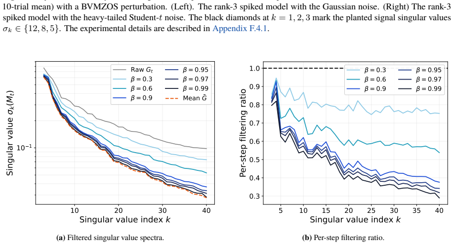
Spectral summaries.Record (i) the singular-value sequences of¯Gand of Pre-polar momentum buffer M (β) K , (ii) the per-step filtering ratioσk(M (β) K )/σk(GK) at the final collection index, and (iii) the noise-suppression ratioR(T) that compares the operator norm of the raw-gradient residual with that of the momentum residual at momentum window sizeT= 1/(...
-
[74]
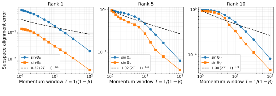
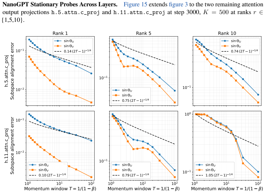
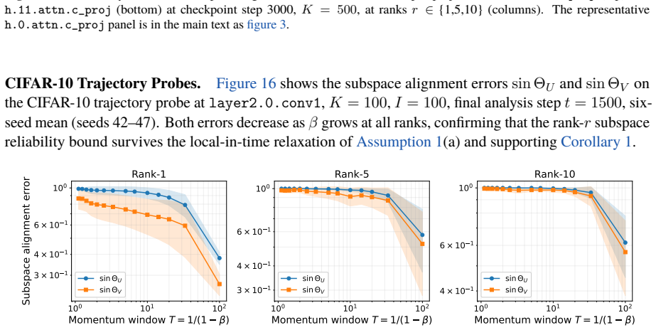
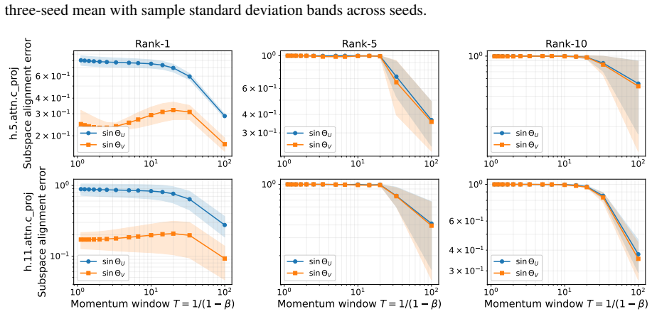
Subspace alignment error panels report thesin Θprincipal-angle distance at fixed ranksr∈{1,5,10}
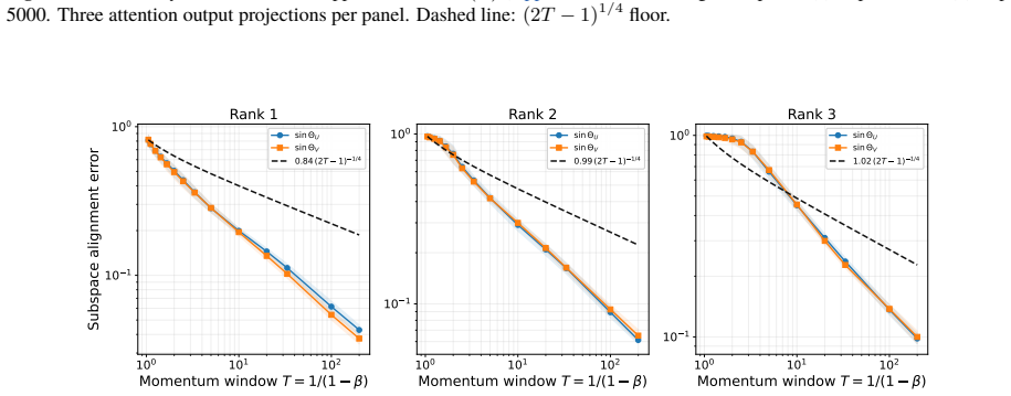
Signal alignment and subspace alignment error metrics.Signal alignment is reported with the rank-r and full-rank signal alignment metricsAlignr and Alignfull of Appendix F.3. Subspace alignment error panels report thesin Θprincipal-angle distance at fixed ranksr∈{1,5,10}. All SVDs inside theAnalysis procedureare exactfloat32 decompositions. Newton–Schulz ...
-
[75]
Per-step filtering ratio— the ratio of thek-th singular value of Pre-polar momentum bufferM (β) K (equation (20)) to that of the latest collected raw gradientGK, Filtk(β) := σk M (β) K σk(GK) . Bothspectraarecomputedfromthesamegradientbufferatthefinalcollectionstep: GK isthelastraw mini-batch gradient (equivalently, the momentum buffer atβ= 0 ), andM (β) ...
-
[76]
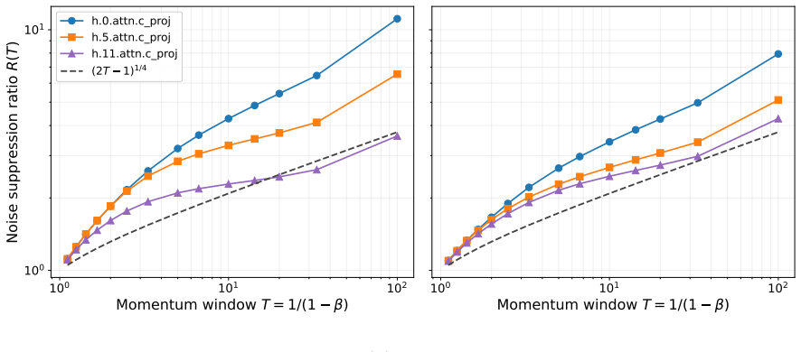
Explicitly, R(T) := GK − ¯G 2 M (β) K − ¯G 2 , ¯G := 1 K KX t=1 Gt, 33 where ¯G is the in-buffer approximation ofGsig t
Noise-suppressionratio—residualoperator-normratio R(T) ofrawgradientvs.Pre-polarmomentum buffer with probe-side momentum coefficientβ (associated with the effective sample size2T−1 ). Explicitly, R(T) := GK − ¯G 2 M (β) K − ¯G 2 , ¯G := 1 K KX t=1 Gt, 33 where ¯G is the in-buffer approximation ofGsig t . Subtracting ¯G from both numerator and denominator ...
-
[77]
Explicitly, sinθ r(A;B) := sin Θ Ur(A), U r(B) 2, with the right-subspace versionsinθ r(A⊤;B ⊤) =∥sin Θ(V r(A), V r(B))∥2 reported separately
Subspace alignment error— thesinθ subspace distance from the top-r singular subspaces of the reference to those of Pre-polar momentum buffer. Explicitly, sinθ r(A;B) := sin Θ Ur(A), U r(B) 2, with the right-subspace versionsinθ r(A⊤;B ⊤) =∥sin Θ(V r(A), V r(B))∥2 reported separately. In this paper, we also definesin ΘU := sinθ r(M (β) K ; ¯G) and sin ΘV :...
-
[78]
Alignr(A;B) := Ur(B)⊤A Vr(B) F√r ∈[0,1]
Signal alignment— the signal alignment comparison applied to Pre-polar=O(M (β) K ), Post-polar = fM (β) K , and Polar-only=O(GK), reported through the following two metrics: Rank-rsignal alignment. Alignr(A;B) := Ur(B)⊤A Vr(B) F√r ∈[0,1]. Larger values indicate stronger signal alignment. Theorem 2 predicts that Pre-polar achieves higher Alignr than Post-p...
2000
-
[79]
Dashed line:(2T−1)1/4 floor
Three attention output projections per panel. Dashed line:(2T−1)1/4 floor. 100 101 102 Momentum window T = 1/(1 ) 10 1 100 Subspace alignment error Rank 1 sin U sin V 0.84 (2T 1) 1/4 100 101 102 Momentum window T = 1/(1 ) 10 1 100 Rank 2 sin U sin V 0.99 (2T 1) 1/4 100 101 102 Momentum window T = 1/(1 ) 10 1 100 Rank 3 sin U sin V 1.02 (2T 1) 1/4 Figure 1...
2000
discussion (0)
Sign in with ORCID, Apple, or X to comment. Anyone can read and Pith papers without signing in.