REVIEW 2 major objections 5 minor 103 references
Fusing heterogeneous data sets
T0 review · 2 major / 5 minor · reviewed 2026-08-14 · deepseek-v4-flash
Pith's one-line read A penalized exponential-family simultaneous component analysis model can fuse binary, count, and quantitative data sets and separate their global-common, local-common, and distinct variation through a group concave penalty on the loading…
desk verdict A coherent PhD thesis compiling four of the author's own methods papers; the P-ESCA chapter is the most original, but the shared-subspace assumption is never stress-tested. read the letter →
The pith
A machine-rendered reading of the paper's core claim, the machinery that carries it, and where it could break.
The reading
What carries the argument
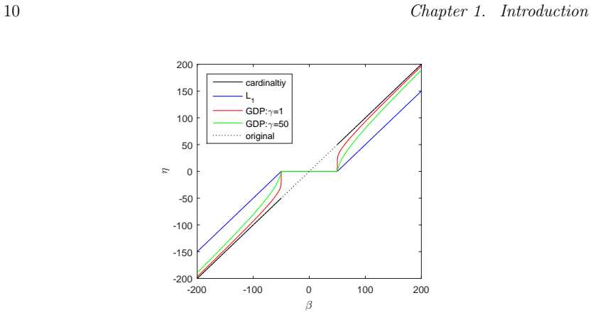
The central object is the loading matrix of an exponential-family simultaneous component analysis model, organized in blocks $B_l$ for each data set. The mechanism is a group concave penalty on these blocks: it shrinks the $\ell^2$ norm of each block nonlinearly, driving small blocks to exactly zero while leaving large blocks nearly unchanged. Those zero blocks create the structured sparsity pattern that identifies which latent components are global, local, or distinct. The fitting machinery is a Majorization-Minimization algorithm that majorizes the negative log-likelihood to a quadratic and the concave penalty to a weighted sum of singular values, yielding closed-form updates that decrease the objective monotonically.
What would settle it
Simulate two data sets with a known shared axis plus a data-set-specific axis, but generate the shared axis with different scaling or through a nonlinear transformation across a binary log-odds scale and a continuous mean scale; if P-ESCA cannot recover the specified common and distinct loading blocks under that generating process, the common-subspace assumption is the point of failure.
Extended reading notes
Core claim
In the ESCA model, the natural parameter matrices of all data sets are assumed to lie in the same column subspace, spanned by a common score matrix $A$, with data-set-specific loadings $B_l$. P-ESCA adds a group concave penalty that acts on the $\ell^2$ norm of each loading block, so whole blocks are shrunk to zero in a nearly unbiased way. The zero blocks mark components that are absent from a given data set, and that pattern is exactly how global, local-common, and distinct variation are read off. A Majorization-Minimization algorithm with closed-form updates fits the penalized likelihood, and a missing-value cross-validation procedure selects the tuning parameters. The paper reports that the method recovers simulated common-distinct structures across mixed data types and illustrates the decomposition on chronic lymphocytic leukaemia data.
Load-bearing premise
The method assumes that the natural parameter matrices of all data sets share exactly the same column subspace, spanned by one common score matrix $A$; if the shared signal is not linearly aligned across measurement scales, or some shared components are weak, the decomposition can be misspecified and the penalty may force the wrong zero blocks.
Editorial extensions
If this is right
- Multiple omics data sets of different measurement scales can be fused in one model without dichotomizing or re-scaling away their distinct natures.
- The loading matrix itself becomes the interpretable map of shared versus unique biology: a zero block means a component is not present in that data set.
- Mixed binary, count, and quantitative data can be integrated for exploratory analysis, with model selection by cross-validation rather than by an ad hoc rank guess.
- Because the algorithm is monotone and has closed-form updates, the approach is computationally tractable in the high-dimensional, low-sample-size settings typical of genomics.
Reading between the lines
- If the common-subspace assumption holds only approximately, the group penalty may still recover the dominant shared axes, but weaker subset-shared components could be forced to zero; a residual-correlation diagnostic between fitted data sets would test this.
- The same block-penalty construction could be combined with element-wise concave penalties to discover partially shared variables, not only wholly shared components, as the thesis itself outlines as a future direction.
- Because each data type is modeled on its natural parameter scale, the estimated common score matrix could plausibly serve as an input to downstream supervised analyses, giving a principled way to use heterogeneous measurements for prediction.
Signed reviews
Editorial analysis
A structured set of objections, weighed in public.
Referee Report
Summary. This manuscript is a PhD thesis on fusing heterogeneous data sets in systems biology. It treats two types of heterogeneity: differences in data type (binary, quantitative, count) and differences in information content (global common, local common, distinct variation). Chapter 2 reviews PCA methods for binary genomics data; Chapter 3 develops a robust logistic PCA via non-convex singular value thresholding; Chapter 4 introduces GSCA for fusing one binary and one quantitative data set; Chapter 5 proposes P-ESCA, an exponential-family simultaneous component analysis with a group concave penalty on the loading matrix to disentangle global, local common, and distinct variation in multiple mixed-type data sets. The main claims are that the MM algorithms are monotonically decreasing, have closed-form updates, that a missing-value cross-validation procedure selects the model, and that simulations and a CLL data analysis support the disentangling claim.
Significance. If the central claims hold, P-ESCA is a potentially useful addition to the multi-block data fusion literature, extending SCA-type decompositions to mixed data types with a structured sparsity pattern. The manuscript gives creditworthy strengths: explicit majorization inequalities, analytic updates for all parameters, monotonicity arguments, a missing-value cross-validation implementation, and comparisons with MOFA and SLIDE in the supplementary material. The simulations are described in enough detail to be reproduced, and the real-data illustration on CLL data shows an applied context. The main weakness is that the disentangling claim rests on a strong shared-subspace assumption that is never stress-tested, and the simulation evidence is generated entirely under that assumption.
major comments (2)
- [§5.2.1] The model assumes that the natural parameter matrices of all data sets lie in exactly the same column subspace spanned by one common score matrix A, i.e., Θ_l = 1μ_l^T + A B_l^T for every block l. This exact equality is load-bearing for the interpretation of zero blocks in B_l as absence of shared variation. If the true data-generating process is not exactly aligned on the linear-predictor scale, for example if a shared biological factor affects the log-odds of binary measurements and the mean of quantitative measurements through different scaling or link functions, or if block-specific rotations are present, then the fitted group concave penalty can shrink blocks to zero to compensate for the misspecification rather than to reveal the true common/distinct structure. Section 5.6 generates data exactly under this model, so the simulations cannot detect such a failure. No misspecification or sensitivity experiment is reported. I recommend adding experiments with perturbed block subspaces, block-specific rotations, or alternative link functions to assess whether the decomposition remains interpretable.
- [§5.6.2] The model selection evaluation for P-ESCA is presented only as an example of CV-error-based selection, not as a systematic evaluation of whether the selected tuning parameters recover the true sparsity pattern. Since the central output of P-ESCA is a structured sparsity pattern that determines which components are global, local common, or distinct, the manuscript should report quantitative agreement between the selected pattern and the true pattern across simulation settings (e.g., varying signal-to-noise ratio, number of blocks, and strength of local common components). This is especially important because earlier chapters show that CV-based selection can behave badly for lasso-type penalties (Chapter 3, nuclear norm) and that the SCAD penalty performs poorly; the reader needs evidence that the group concave penalty does not inherit these problems in the multi-block setting.
minor comments (5)
- [§4.3.1] The heading 'The majorization of the penalized negative lilkelihood' contains a typo: 'lilkelihood' should be 'likelihood'.
- [§4.5.2] In the sentence beginning 'using the GCSA model's CNA loadings', 'GCSA' should be 'GSCA' to match the model name used elsewhere.
- [§5.5] The section title 'Evaluation matrices and model selection' should probably read 'Evaluation metrics and model selection'.
- [Chapter 1] In the sentence about multiple score and loading vectors, 'vcectors' should be 'vectors'.
- [General] The thesis is composed of chapters that are based on previously published or preprint papers. If this is submitted as a journal article, the new contribution of Chapter 5 should be clearly delineated from the published material in Chapters 2–4, and the manuscript should be restructured into a self-contained article.
Circularity Check
No significant circularity: the derivation chain is self-contained and simulations are self-consistency checks, not predictions forced by construction.
full rationale
The thesis develops statistical methods (logistic PCA variants, GSCA, P-ESCA) and evaluates them by simulation and real-data illustration. No step in the derivation chain uses the target result as an input. The P-ESCA model assumes that the natural parameter matrices lie in a common column subspace spanned by A; this is a model assumption, not a derived conclusion about biology, and the paper does not claim to derive that assumption from the data. The structured sparsity pattern in the loading matrix is the model's definition of global-common, local-common, and distinct variation; the claim is that the group concave penalty can recover such a pattern, which is a methodological claim supported by simulations that generate data from the same model family and then check parameter recovery. That is a standard self-consistency check, not circular prediction: the generative values are known, and the fitted model is not constructed to equal them by definition. The thesis chapters are based on the author's own prior papers, but this is ordinary thesis compilation; the cited prior work is not used to justify a conclusion that would otherwise lack support. The measurement-scale uniqueness theorem in Chapter 1 is an external result, not imported from the authors. Concerns about misspecification when the shared signal is not exactly aligned across data types are model-assumption risks, not circularity. No fitted parameter is renamed as a prediction, and no uniqueness theorem from the authors' own work is invoked to forbid alternatives. The derivations of the MM algorithms are explicit and do not presuppose the numerical results reported.
Assumptions & free parameters
free parameters (4)
- m (saturated-model log-odds approximation) =
2.94
- lambda (penalty strength) =
selected by cross-validation
- gamma (GDP penalty hyper-parameter) =
default 1; grid searched in Chapter 3
- R (low rank / number of components) =
selected by CV; known in simulations
assumptions (5)
- domain assumption Elements of each data set are conditionally independent given the natural parameter matrix and link function.
- domain assumption The true data generation in simulations follows the same logistic PCA or exponential-family SCA models being tested.
- domain assumption The common score matrix A spans the same column subspace for all data sets in GSCA and P-ESCA.
- standard math The proximal operator for weighted singular value thresholding has the closed form used in the algorithms.
- standard math The MM majorization with Lipschitz constant L=0.25 for the logit negative log-likelihood is valid.
Cite this review
Pith. "Pith review of Fusing heterogeneous data sets." pith.science (2026). https://pith.science/paper/5SAQQZOU
@misc{pith2026190809653,
  author       = {Pith},
  title        = {Pith review of: Fusing heterogeneous data sets},
  year         = {2026},
  howpublished = {\url{https://pith.science/paper/5SAQQZOU}},
  note         = {Machine review of arXiv:1908.09653}
}
read the original abstract
In systems biology, it is common to measure biochemical entities at different levels of the same biological system. One of the central problems for the data fusion of such data sets is the heterogeneity of the data. This thesis discusses two types of heterogeneity. The first one is the type of data, such as metabolomics, proteomics and RNAseq data in genomics. These different omics data reflect the properties of the studied biological system from different perspectives. The second one is the type of scale, which indicates the measurements obtained at different scales, such as binary, ordinal, interval and ratio-scaled variables. In this thesis, we developed several statistical methods capable to fuse data sets of these two types of heterogeneity. The advantages of the proposed methods in comparison with other approaches are assessed using comprehensive simulations as well as the analysis of real biological data sets.
Figures


Figures from the paper (33 more)


Reference graph
Works this paper leans on
-
[1]
Integration of metabolomics and transcriptomics reveals a complex diet of mycobacterium tuberculosis during early macrophage infection,
M. Zimmermann, M. Kogadeeva, M. Gengenbacher, G. McEwen, H.-J. Mol- lenkopf, N. Zamboni, S. H. E. Kaufmann, and U. Sauer, “Integration of metabolomics and transcriptomics reveals a complex diet of mycobacterium tuberculosis during early macrophage infection,” mSystems, vol. 2, no. 4, pp. e00057–17, 2017
2017
-
[2]
A methodology for sensor fusion design: Application to fruit quality assessment,
V. Steinmetz, F. Sevila, and V. Bellon-Maurel, “A methodology for sensor fusion design: Application to fruit quality assessment,” Journal of Agricul- tural Engineering Research, vol. 74, no. 1, pp. 21–31, 1999
1999
-
[3]
On the increase of predictive performance with high-level data fusion,
T. Doeswijk, A. Smilde, J. Hageman, J. Westerhuis, and F. Van Eeuwijk, “On the increase of predictive performance with high-level data fusion,” Analytica Chimica Acta, vol. 705, no. 1-2, pp. 41–47, 2011
2011
-
[4]
On the theory of scales of measurement,
S. Stevens, “On the theory of scales of measurement,” Science, vol. 103, pp. 677–680, June 1946
1946
-
[5]
Basic measurement theory,
P. Suppes and J. Zinnes, “Basic measurement theory,” Psychology Series 45, Stanford University, Institute for Mathematical Studies in the Social Sci- ences, March 1962
1962
-
[6]
Krantz, R
D. Krantz, R. Luce, P. Suppes, and A. Tversky, Foundations of Measure- ment (Volume I). Dover, 1971
1971
-
[7]
On the scales of measurement,
L. Narens, “On the scales of measurement,” Journal of Mathematical Psy- chology, vol. 24, no. 3, pp. 249–275, 1981
1981
-
[8]
Measurement - the theory of numerical assign- ments,
L. Narens and R. D. Luce, “Measurement - the theory of numerical assign- ments,” Psychological Bulletin, vol. 99, pp. 166–180, Mar. 1986
1986
Show all 103 references
-
[9]
Measurement scales on the continuum,
R. D. Luce and L. Narens, “Measurement scales on the continuum,”Science, vol. 236, no. 4808, pp. 1527–1532, 1987. 155 156 Bibliography
1987
-
[10]
Statistics and the theory of measurement,
D. J. Hand, “Statistics and the theory of measurement,” Journal of the Royal Statistical Society Series A-statistics in Society , vol. 159, pp. 445– 473, 1996
1996
-
[11]
A theory of appropriate statistics,
E. Adams, R. Fagot, and R. Robinson, “A theory of appropriate statistics,” Psychometrika, vol. 30, no. 2, pp. 99–127, 1965
1965
-
[12]
Measurement scales and statistics - a clash of paradigms,
J. Michell, “Measurement scales and statistics - a clash of paradigms,” Psychological Bulletin, vol. 100, no. 3, pp. 398–407, 1986
1986
-
[13]
Agresti, Categorical data analysis
A. Agresti, Categorical data analysis. John Wiley & Sons, 2013
2013
-
[14]
Common and distinct components in data fusion,
A. K. Smilde, I. M˚ age, T. Naes, T. Hankemeier, M. A. Lips, H. A. Kiers, E. Acar, and R. Bro, “Common and distinct components in data fusion,” Journal of Chemometrics , vol. 31, no. 7, p. e2900, 2017
2017
-
[15]
Structural learning and integrative decomposition of multi-view data,
I. Gaynanova and G. Li, “Structural learning and integrative decomposition of multi-view data,” arXiv preprint arXiv:1707.06573 , 2017
2017 arXiv
-
[16]
Variable selection via nonconcave penalized likelihood and its oracle properties,
J. Fan and R. Li, “Variable selection via nonconcave penalized likelihood and its oracle properties,” Journal of the American Statistical Association , vol. 96, no. 456, pp. 1348–1360, 2001
2001
-
[17]
Jolliffe, Principal component analysis
I. Jolliffe, Principal component analysis. Wiley Online Library, 2002
2002
-
[18]
Optimal shrinkage of singular values,
M. Gavish and D. L. Donoho, “Optimal shrinkage of singular values,” IEEE Transactions on Information Theory, vol. 63, no. 4, pp. 2137–2152, 2017
2017
-
[19]
Sparse inverse covariance esti- mation with the graphical lasso,
J. Friedman, T. Hastie, and R. Tibshirani, “Sparse inverse covariance esti- mation with the graphical lasso,” Biostatistics, vol. 9, no. 3, pp. 432–441, 2008
2008
-
[20]
Sparsity and smoothness via the fused lasso,
R. Tibshirani, M. Saunders, S. Rosset, J. Zhu, and K. Knight, “Sparsity and smoothness via the fused lasso,”Journal of the Royal Statistical Society: Series B (Statistical Methodology) , vol. 67, no. 1, pp. 91–108, 2005
2005
-
[21]
A penalized matrix decom- position, with applications to sparse principal components and canonical correlation analysis,
D. M. Witten, R. Tibshirani, and T. Hastie, “A penalized matrix decom- position, with applications to sparse principal components and canonical correlation analysis,” Biostatistics, vol. 10, no. 3, pp. 515–534, 2009
2009
-
[22]
A selective review of group selection in high-dimensional models,
J. Huang, P. Breheny, and S. Ma, “A selective review of group selection in high-dimensional models,” Statistical Science: A Review Journal of The Institute of Mathematical Statistics , vol. 27, no. 4, 2012
2012
-
[23]
Regression shrinkage and selection via the lasso,
R. Tibshirani, “Regression shrinkage and selection via the lasso,” Journal of the Royal Statistical Society: Series B (Methodological) , vol. 58, no. 1, pp. 267–288, 1996. Bibliography 157
1996
-
[24]
Least angle regres- sion,
B. Efron, T. Hastie, I. Johnstone, R. Tibshirani, et al., “Least angle regres- sion,” The Annals of Statistics , vol. 32, no. 2, pp. 407–499, 2004
2004
-
[25]
Proximal algorithms,
N. Parikh, S. Boyd, et al. , “Proximal algorithms,” Foundations and Trends R© in Optimization, vol. 1, no. 3, pp. 127–239, 2014
2014
-
[26]
Stability selection,
N. Meinshausen and P. B¨ uhlmann, “Stability selection,” Journal of the Royal Statistical Society: Series B (Statistical Methodology) , vol. 72, no. 4, pp. 417–473, 2010
2010
-
[27]
Generalized double Pareto shrink- age,
A. Armagan, D. B. Dunson, and J. Lee, “Generalized double Pareto shrink- age,” Statistica Sinica, vol. 23, no. 1, p. 119, 2013
2013
-
[28]
Performance of meth- ods that separate common and distinct variation in multiple data blocks,
I. M˚ age, A. K. Smilde, and F. M. van der Kloet, “Performance of meth- ods that separate common and distinct variation in multiple data blocks,” Journal of Chemometrics , vol. 33, no. 1, p. e3085, 2019
2019
-
[29]
Comprehensive genomic characterization defines human glioblastoma genes and core pathways,
C. G. A. T. R. Network et al. , “Comprehensive genomic characterization defines human glioblastoma genes and core pathways,” Nature, vol. 455, no. 7216, pp. 1061–1068, 2008
2008
-
[30]
A landscape of pharmacogenomic interactions in cancer,
F. Iorio, T. A. Knijnenburg, D. J. Vis, G. R. Bignell, M. P. Menden, M. Schubert, N. Aben, E. Gon¸ calves, S. Barthorpe, H. Lightfoot, et al. , “A landscape of pharmacogenomic interactions in cancer,” Cell, vol. 166, no. 3, pp. 740–754, 2016
2016
-
[31]
Detecting independent and recurrent copy number aberrations using interval graphs,
H.-T. Wu, I. Hajirasouliha, and B. J. Raphael, “Detecting independent and recurrent copy number aberrations using interval graphs,” Bioinformatics, vol. 30, pp. i195–i203, June 2014
2014
-
[32]
Quantifying qualitative data,
F. W. Young, J. de Leeuw, and Y. Takane, “Quantifying qualitative data,” Lantermann and H. Feger (Eds.): Similarity and Choice. Papers in Honour of Clyde Coombs. Berne: Hans Huber , 1980
1980
-
[33]
A generalization of princi- pal component analysis to the exponential family,
M. Collins, S. Dasgupta, and R. E. Schapire, “A generalization of princi- pal component analysis to the exponential family,” in Advances in Neural Information Processing Systems, MIT Press, 2001
2001
-
[34]
A generalized linear model for principal component analysis of binary data.,
A. I. Schein, L. K. Saul, and L. H. Ungar, “A generalized linear model for principal component analysis of binary data.,” in AISTATS, vol. 3, p. 10, 2003
2003
-
[35]
A. J. Landgraf, Generalized principal component analysis: Dimensionality reduction through the projection of natural parameters . PhD thesis, The Ohio State University, 2015. 158 Bibliography
2015
-
[36]
Gifi methods for optimal scaling in R: the package homals,
J. de Leeuw and P. Mair, “Gifi methods for optimal scaling in R: the package homals,” Journal of Statistical Software , vol. 31, pp. 1–21, AUG 2009
2009
-
[37]
Y. Mori, M. Kuroda, and N. Makino, Nonlinear principal component anal- ysis and its applications . Springer, 2016
2016
-
[38]
H. A. Kiers, Three-way methods for the analysis of qualitative and quanti- tative two-way data . DSWO press Leiden, 1989
1989
-
[39]
On lines and planes of closest fit to systems of points in space,
K. Pearson, “On lines and planes of closest fit to systems of points in space,” Philosophical Magazine Series 6 , vol. 2, no. 11, pp. 559–572, 1901
1901
-
[40]
Sparse principal component anal- ysis,
H. Zou, T. Hastie, and R. Tibshirani, “Sparse principal component anal- ysis,” Journal of Computational and Graphical Statistics , vol. 15, no. 2, pp. 265–286, 2006
2006
-
[41]
J. M. ten Berge, Least squares optimization in multivariate analysis. DSWO Press, Leiden University Leiden, 1993
1993
-
[42]
Probabilistic principal component anal- ysis,
M. E. Tipping and C. M. Bishop, “Probabilistic principal component anal- ysis,” Journal of the Royal Statistical Society: Series B (Statistical Method- ology), vol. 61, no. 3, pp. 611–622, 1999
1999
-
[43]
Principal component analysis of binary data by iterated singular value decomposition,
J. De Leeuw, “Principal component analysis of binary data by iterated singular value decomposition,” Computational Statistics & Data analysis , vol. 50, no. 1, pp. 21–39, 2006
2006
-
[44]
Generalized low rank models,
M. Udell, C. Horn, R. Zadeh, et al., “Generalized low rank models,” Foun- dations and Trends R© in Machine Learning, vol. 9, no. 1, pp. 1–118, 2016
2016
-
[45]
Gifi, Nonlinear multivariate analysis
A. Gifi, Nonlinear multivariate analysis . New York, N.Y.: Wiley, 1990. This is a publication under a collective pseudonym
1990
-
[46]
The role of balanced training and testing data sets for binary classifiers in bioinformatics,
Q. Wei and R. L. Dunbrack Jr, “The role of balanced training and testing data sets for binary classifiers in bioinformatics,” PloS One , vol. 8, no. 7, p. e67863, 2013
2013
-
[47]
Cross-validatory estimation of the number of components in factor and principal components models,
S. Wold, “Cross-validatory estimation of the number of components in factor and principal components models,” Technometrics, vol. 20, no. 4, pp. 397–405, 1978
1978
-
[48]
Cross-validation of component models: A critical look at current methods,
R. Bro, K. Kjeldahl, A. K. Smilde, et al., “Cross-validation of component models: A critical look at current methods,” Analytical and Bioanalytical Chemistry, vol. 390, no. 5, pp. 1241–1251, 2008
2008
-
[49]
R Foundation for Statistical Computing, Vienna, Austria, 2008
R Development Core Team, R: A language and environment for statistical computing. R Foundation for Statistical Computing, Vienna, Austria, 2008. ISBN 3-900051-07-0. Bibliography 159
2008
-
[50]
pcaMethods–a bioconduc- tor package providing PCA methods for incomplete data,
W. Stacklies, H. Redestig, M. Scholz, et al. , “pcaMethods–a bioconduc- tor package providing PCA methods for incomplete data,” Bioinformatics, vol. 23, no. 9, pp. 1164–1167, 2007
2007
-
[51]
Multinomial multiple correspondence analy- sis,
P. J. Groenen and J. Josse, “Multinomial multiple correspondence analy- sis,” arXiv preprint arXiv:1603.03174 , 2016
2016 arXiv
-
[52]
1-Bit matrix completion,
M. A. Davenport, Y. Plan, E. Van Den Berg, and M. Wootters, “1-Bit matrix completion,” Information and Inference: A Journal of the IMA , vol. 3, no. 3, pp. 189–223, 2014
2014
-
[53]
Reconstruction of a low-rank matrix in the presence of gaussian noise,
A. A. Shabalin and A. B. Nobel, “Reconstruction of a low-rank matrix in the presence of gaussian noise,” Journal of Multivariate Analysis , vol. 118, pp. 67–76, 2013
2013
-
[54]
Adaptive shrinkage of singular values,
J. Josse and S. Sardy, “Adaptive shrinkage of singular values,” Statistics and Computing, vol. 26, no. 3, pp. 715–724, 2016
2016
-
[55]
Exact matrix completion via convex optimiza- tion,
E. J. Cand` es and B. Recht, “Exact matrix completion via convex optimiza- tion,” Foundations of Computational Mathematics , vol. 9, no. 6, p. 717, 2009
2009
-
[56]
Spectral regularization algo- rithms for learning large incomplete matrices,
R. Mazumder, T. Hastie, and R. Tibshirani, “Spectral regularization algo- rithms for learning large incomplete matrices,”Journal of Machine Learning Research, vol. 11, no. Aug, pp. 2287–2322, 2010
2010
-
[57]
Penalized regressions: The bridge versus the lasso,
W. J. Fu, “Penalized regressions: The bridge versus the lasso,” Journal of Computational and Graphical Statistics , vol. 7, no. 3, pp. 397–416, 1998
1998
-
[58]
Block-relaxation algorithms in statistics,
J. De Leeuw, “Block-relaxation algorithms in statistics,” in Information Systems and Data Analysis , pp. 308–324, Springer, 1994
1994
-
[59]
A tutorial on MM algorithms,
D. R. Hunter and K. Lange, “A tutorial on MM algorithms,” The American Statistician, vol. 58, no. 1, pp. 30–37, 2004
2004
-
[60]
Weighted least squares fitting using ordinary least squares algorithms,
H. A. L. Kiers, “Weighted least squares fitting using ordinary least squares algorithms,” Psychometrika, vol. 62, no. 2, pp. 251–266, 1997
1997
-
[61]
Boyd and L
S. Boyd and L. Vandenberghe, Convex optimization. Cambridge University Press, 2004
2004
-
[62]
Generalized singular value thresholding,
C. Lu, C. Zhu, C. Xu, S. Yan, and Z. Lin, “Generalized singular value thresholding,” in Twenty-Ninth AAAI Conference on Artificial Intelligence, 2015
2015
-
[63]
Le Cam and G
L. Le Cam and G. L. Yang, Asymptotics in statistics: Some basic concepts . Springer Science and Business Media, 2012. 160 Bibliography
2012
-
[64]
Generalized simultaneous component analysis of binary and quantitative data,
Y. Song, J. A. Westerhuis, N. Aben, L. F. Wessels, P. J. Groenen, and A. K. Smilde, “Generalized simultaneous component analysis of binary and quantitative data,” arXiv preprint arXiv:1807.04982 , 2018
2018 arXiv
-
[65]
A structured overview of simultaneous component based data integration,
K. Van Deun, A. K. Smilde, M. J. van der Werf, H. A. L. Kiers, and I. Van Mechelen, “A structured overview of simultaneous component based data integration,” BMC Bioinformatics, vol. 10, no. 1, p. 246, 2009
2009
-
[66]
Integrating functional genomics data using maximum likelihood based simultaneous component analysis,
R. A. van den Berg, I. Van Mechelen, T. F. Wilderjans, K. Van Deun, H. A. L. Kiers, and A. K. Smilde, “Integrating functional genomics data using maximum likelihood based simultaneous component analysis,” BMC Bioinformatics, vol. 10, no. 1, p. 340, 2009
2009
-
[67]
Pattern discovery and cancer gene iden- tification in integrated cancer genomic data,
Q. Mo, S. Wang, V. E. Seshan, A. B. Olshen, N. Schultz, C. Sander, R. S. Powers, M. Ladanyi, and R. Shen, “Pattern discovery and cancer gene iden- tification in integrated cancer genomic data,” Proceedings of the National Academy of Sciences, vol. 110, no. 11, pp. 4245–4250, 2013
2013
-
[68]
A generalization of princi- pal components analysis to the exponential family,
M. Collins, S. Dasgupta, and R. E. Schapire, “A generalization of princi- pal components analysis to the exponential family,” in Advances in Neural Information Processing Systems, pp. 617–624, 2002
2002
-
[69]
Nuclear-norm penaliza- tion and optimal rates for noisy low-rank matrix completion,
V. Koltchinskii, K. Lounici, A. B. Tsybakov, et al., “Nuclear-norm penaliza- tion and optimal rates for noisy low-rank matrix completion,” The Annals of Statistics, vol. 39, no. 5, pp. 2302–2329, 2011
2011
-
[70]
Fast dimension reduction and integrative clustering of multi-omics data using low-rank approximation: Application to cancer molecular classification,
D. Wu, D. Wang, M. Q. Zhang, and J. Gu, “Fast dimension reduction and integrative clustering of multi-omics data using low-rank approximation: Application to cancer molecular classification,” BMC Genomics , vol. 16, no. 1, p. 1022, 2015
2015
-
[71]
Cross-validation of component models: A critical look at current methods,
R. Bro, K. Kjeldahl, A. K. Smilde, and H. A. L. Kiers, “Cross-validation of component models: A critical look at current methods,” Analytical and Bioanalytical Chemistry, vol. 390, no. 5, pp. 1241–1251, 2008
2008
-
[72]
Support vector machines with adaptive Lq penalty,
Y. Liu, H. H. Zhang, C. Park, and J. Ahn, “Support vector machines with adaptive Lq penalty,” Computational Statistics & Data Analysis , vol. 51, no. 12, pp. 6380–6394, 2007
2007
-
[73]
Principal component analysis of binary genomics data,
Y. Song, J. A. Westerhuis, N. Aben, M. Michaut, L. F. Wessels, and A. K. Smilde, “Principal component analysis of binary genomics data,” Briefings in Bioinformatics, 2017
2017
-
[74]
Genomic classifica- tion of cutaneous melanoma,
R. Akbani, K. C. Akdemir, B. A. Aksoy, M. Albert, A. Ally, S. B. Amin, H. Arachchi, A. Arora, J. T. Auman, B. Ayala, et al., “Genomic classifica- tion of cutaneous melanoma,” Cell, vol. 161, no. 7, pp. 1681–1696, 2015. Bibliography 161
2015
-
[75]
Comprehensive molecular profiling of lung adenocarcinoma,
C. G. A. R. Network et al. , “Comprehensive molecular profiling of lung adenocarcinoma,” Nature, vol. 511, no. 7511, p. 543, 2014
2014
-
[76]
Comprehensive molecular portraits of human breast tumours,
C. G. A. Network et al. , “Comprehensive molecular portraits of human breast tumours,” Nature, vol. 490, no. 7418, p. 61, 2012
2012
-
[77]
iTOP: Inferring the topology of omics data,
N. Aben, J. A. Westerhuis, Y. Song, H. A. L. Kiers, M. Michaut, A. K. Smilde, and L. F. A. Wessels, “iTOP: Inferring the topology of omics data,” Bioinformatics, vol. 34, pp. i988–i996, 09 2018
2018
-
[78]
Learning the structure of mixed graphical models,
J. D. Lee and T. J. Hastie, “Learning the structure of mixed graphical models,” Journal of Computational and Graphical Statistics , vol. 24, no. 1, pp. 230–253, 2015
2015
-
[79]
High-dimensional mixed graphical models,
J. Cheng, T. Li, E. Levina, and J. Zhu, “High-dimensional mixed graphical models,” Journal of Computational and Graphical Statistics , vol. 26, no. 2, pp. 367–378, 2017
2017
-
[80]
Integrative clustering of multiple genomic data types using a joint latent variable model with application to breast and lung cancer subtype analysis,
R. Shen, A. B. Olshen, and M. Ladanyi, “Integrative clustering of multiple genomic data types using a joint latent variable model with application to breast and lung cancer subtype analysis,” Bioinformatics, vol. 25, no. 22, pp. 2906–2912, 2009
2009
-
[81]
Separating common from distinctive variation,
F. M. van der Kloet, P. Sebasti´ an-Le´ on, A. Conesa, A. K. Smilde, and J. A. Westerhuis, “Separating common from distinctive variation,” BMC bioinformatics, vol. 17, no. 5, p. S195, 2016
2016
-
[82]
Joint and individual variation explained (JIVE) for integrated analysis of multiple data types,
E. F. Lock, K. A. Hoadley, J. S. Marron, and A. B. Nobel, “Joint and individual variation explained (JIVE) for integrated analysis of multiple data types,” The Annals of Applied Statistics , vol. 7, no. 1, p. 523, 2013
2013
-
[83]
Global, local and unique decom- positions in OnPLS for multiblock data analysis,
T. L¨ ofstedt, D. Hoffman, and J. Trygg, “Global, local and unique decom- positions in OnPLS for multiblock data analysis,” Analytica Chimica Acta, vol. 791, pp. 13–24, 2013
2013
-
[84]
Performing DISCO-SCA to search for distinctive and common information in linked data,
M. Schouteden, K. Van Deun, T. F. Wilderjans, and I. Van Mechelen, “Performing DISCO-SCA to search for distinctive and common information in linked data,” Behavior Research Methods , vol. 46, no. 2, pp. 576–587, 2014
2014
-
[85]
Preference mapping by PO-PLS: Separating common and unique information in several data blocks,
I. M˚ age, E. Menichelli, and T. Næs, “Preference mapping by PO-PLS: Separating common and unique information in several data blocks,” Food Quality and Preference, vol. 24, no. 1, pp. 8–16, 2012
2012
-
[86]
Performance of meth- ods that separate common and distinct variation in multiple data blocks,
I. M˚ age, A. K. Smilde, and F. M. van der Kloet, “Performance of meth- ods that separate common and distinct variation in multiple data blocks,” Journal of Chemometrics , p. e3085, 2018. 162 Bibliography
2018
-
[87]
Group factor analy- sis,
A. Klami, S. Virtanen, E. Lepp¨ aaho, and S. Kaski, “Group factor analy- sis,” IEEE Transactions on Neural Networks and Learning Systems, vol. 26, no. 9, pp. 2136–2147, 2015
2015
-
[88]
Cross-validation for unsupervised learning,
P. O. Perry, “Cross-validation for unsupervised learning,” arXiv preprint arXiv:0909.3052, 2009
2009 arXiv
-
[89]
Multi-Omics Factor Analysis—a framework for unsupervised integration of multi-omics data sets,
R. Argelaguet, B. Velten, D. Arnol, S. Dietrich, T. Zenz, J. C. Marioni, F. Buettner, W. Huber, and O. Stegle, “Multi-Omics Factor Analysis—a framework for unsupervised integration of multi-omics data sets,”Molecular Systems Biology, vol. 14, no. 6, p. e8124, 2018
2018
-
[90]
High-dimensional graphs and vari- able selection with the lasso,
N. Meinshausen, P. B¨ uhlmann,et al., “High-dimensional graphs and vari- able selection with the lasso,” The Annals of Statistics , vol. 34, no. 3, pp. 1436–1462, 2006
2006
-
[91]
A note on the lasso and related procedures in model selection,
C. Leng, Y. Lin, and G. Wahba, “A note on the lasso and related procedures in model selection,” Statistica Sinica, pp. 1273–1284, 2006
2006
-
[92]
Drug-perturbation- based stratification of blood cancer,
S. Dietrich, M. Ole´ s, J. Lu, L. Sellner, S. Anders, B. Velten, B. Wu, J. H¨ ullein, M. da Silva Liberio, T. Walther, et al. , “Drug-perturbation- based stratification of blood cancer,” The Journal of Clinical Investigation , vol. 128, no. 1, pp. 427–445, 2018
2018
-
[93]
A flexible framework for sparse simultaneous component based data integration,
K. Van Deun, T. F. Wilderjans, R. A. Van den Berg, A. Antoniadis, and I. Van Mechelen, “A flexible framework for sparse simultaneous component based data integration,” BMC Bioinformatics, vol. 12, no. 1, p. 448, 2011
2011
-
[94]
Data fusion in metabolomics using cou- pled matrix and tensor factorizations,
E. Acar, R. Bro, and A. K. Smilde, “Data fusion in metabolomics using cou- pled matrix and tensor factorizations,” Proceedings of the IEEE , vol. 103, no. 9, pp. 1602–1620, 2015
2015
-
[95]
Logistic principal compo- nent analysis via non-convex singular value thresholding,
Y. Song, J. A. Westerhuis, and A. K. Smilde, “Logistic principal compo- nent analysis via non-convex singular value thresholding,” arXiv preprint arXiv:1902.09486, 2019
1902 arXiv
-
[96]
Gelman, H
A. Gelman, H. S. Stern, J. B. Carlin, D. B. Dunson, A. Vehtari, and D. B. Rubin, Bayesian data analysis . Chapman and Hall/CRC, 2013
2013
-
[97]
Ma- trix correlations for high-dimensional data: the modified RV-coefficient,
A. K. Smilde, H. A. Kiers, S. Bijlsma, C. Rubingh, and M. Van Erk, “Ma- trix correlations for high-dimensional data: the modified RV-coefficient,” Bioinformatics, vol. 25, no. 3, pp. 401–405, 2008
2008
-
[98]
A tutorial on bayesian optimization,
P. I. Frazier, “A tutorial on bayesian optimization,” arXiv preprint arXiv:1807.02811, 2018. Bibliography 163
2018 arXiv
-
[99]
Practical bayesian optimiza- tion of machine learning algorithms,
J. Snoek, H. Larochelle, and R. P. Adams, “Practical bayesian optimiza- tion of machine learning algorithms,” in Advances in Neural Information Processing Systems, pp. 2951–2959, 2012
2012
-
[100]
Distributed optimization and statistical learning via the alternating direction method of multipliers,
S. Boyd, N. Parikh, E. Chu, B. Peleato, J. Eckstein, et al. , “Distributed optimization and statistical learning via the alternating direction method of multipliers,” Foundations and Trends R© in Machine learning , vol. 3, no. 1, pp. 1–122, 2011
2011
-
[101]
XPCA: Ex- tending PCA for a combination of discrete and continuous variables,
C. Anderson-Bergman, T. G. Kolda, and K. Kincher-Winoto, “XPCA: Ex- tending PCA for a combination of discrete and continuous variables,”arXiv preprint arXiv:1808.07510, 2018
2018 arXiv
-
[102]
Partial least-squares regression: a tutorial,
P. Geladi and B. R. Kowalski, “Partial least-squares regression: a tutorial,” Analytica Chimica Acta, vol. 185, pp. 1–17, 1986
1986
-
[103]
ANOVA-simultaneous component anal- ysis (ASCA): a new tool for analyzing designed metabolomics data,
A. K. Smilde, J. J. Jansen, H. C. Hoefsloot, R.-J. A. Lamers, J. Van Der Greef, and M. E. Timmerman, “ANOVA-simultaneous component anal- ysis (ASCA): a new tool for analyzing designed metabolomics data,” Bioin- formatics, vol. 21, no. 13, pp. 3043–3048, 2005
2005
Reviewed August 14, 2026 · model on record in the stance chip above.
Discussion (0). Continue with ORCID to comment.