Distributed Continuous-Time Control via System Level Synthesis
Pith reviewed 2026-05-23 18:49 UTC · model grok-4.3
The pith
Extending system level synthesis to continuous time yields distributed controllers whose H2 and H-infinity performance matches that of optimal centralized designs while allowing only local communication and local disturbance rejection.
A machine-rendered reading of the paper's core claim, the machinery that carries it, and where it could break.
Core claim
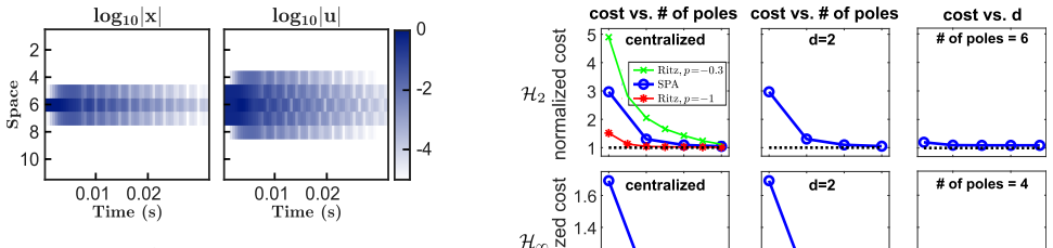
By extending the system level synthesis parameterization to continuous time and applying a pole-selection step followed by an optimization step, the authors obtain distributed H2 and H-infinity controllers that, on the nine-node linearized swing-equation network, achieve costs comparable to the optimal centralized controllers while enforcing local disturbance rejection and local communication.
What carries the argument
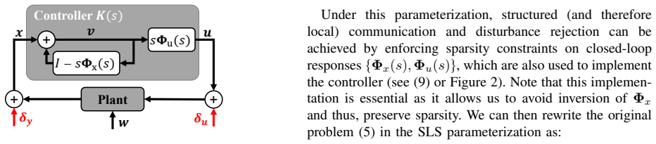
The continuous-time system level synthesis parameterization, which directly parameterizes the closed-loop response maps and thereby converts distributed controller design into a convex optimization problem subject to locality constraints.
If this is right
- Controllers synthesized this way reject disturbances that affect only a local subset of nodes without propagating the effect across the entire network.
- The same parameterization works for both H2 and H-infinity objectives under the locality constraints.
- The method applies directly to any continuous-time linear system once the closed-loop poles have been chosen.
- Local communication patterns are preserved by construction because the SLS maps are constrained to respect the communication graph.
Where Pith is reading between the lines
- The approach could be tested on networks whose size exceeds what centralized solvers can handle, to check whether the locality constraints remain feasible at scale.
- If the pole-selection step can be automated or made robust to model uncertainty, the procedure would become fully data-driven.
- The same continuous-time SLS maps might be combined with model-predictive or learning-based outer loops to handle nonlinear or time-varying dynamics.
Load-bearing premise
The system level synthesis parameterization remains a valid and complete description of all stabilizing controllers when the underlying dynamics are continuous-time linear systems.
What would settle it
On the nine-node grid example, if any distributed controller produced by the two-step procedure either fails to stabilize the closed-loop system or yields an H2 or H-infinity cost more than a few percent above the centralized optimum, the central claim would be refuted.
Figures

read the original abstract
This paper designs H2 and H-infinity distributed controllers with local communication and local disturbance rejection. We propose a two-step procedure: first, select closed-loop poles; then, optimize over parameterized controllers. We build on the system level synthesis (SLS) parameterization -- primarily used in the discrete-time setting -- and extend it to the general continuous-time setting. We verify our approach in simulation on a 9-node grid governed by linearized swing equations, where our distributed controllers achieve performance comparable to that of optimal centralized controllers while facilitating local disturbance rejection.
Editorial analysis
A structured set of objections, weighed in public.
Referee Report
Summary. The paper extends the system level synthesis (SLS) parameterization from discrete to continuous time and proposes a two-step design procedure (closed-loop pole selection followed by convex optimization over the parameterized maps) to synthesize distributed H2 and H∞ controllers that respect a given communication graph and achieve local disturbance rejection. The method is illustrated on a 9-node network whose dynamics are given by linearized swing equations; the resulting distributed controllers are reported to achieve performance comparable to the optimal centralized controller.
Significance. A valid continuous-time SLS parameterization that preserves convexity, locality, and internal stability would supply a convex-optimization route to distributed controller synthesis for continuous-time plants, which is relevant for power-system and networked-control applications. The simulation result, if supported by quantitative norm comparisons, would indicate that the locality constraints need not incur large performance loss relative to the centralized optimum.
major comments (3)
- [Abstract / §2] The central claim rests on the assertion that the SLS closed-loop map parameterization extends to the general continuous-time setting while retaining convexity and the Youla-type property that guarantees internal stability. No derivation, state-space realization, or reference establishing the continuous-time maps (e.g., the continuous-time analogues of the discrete-time Φ11, Φ12, Φ21, Φ22) is supplied, leaving the load-bearing extension unverified.
- [Abstract / §3] The two-step procedure (pole selection then optimization) is stated to produce stabilizing distributed controllers, yet the manuscript provides no argument showing that an arbitrary choice of closed-loop poles, once inserted into the localized SLS parameterization, yields a controller that internally stabilizes the continuous-time plant under the imposed communication-graph constraint. This interaction is load-bearing for both stability and the performance claims.
- [Simulation results] Table or figure reporting the 9-node grid results: the claim of “performance comparable to that of optimal centralized controllers” is not accompanied by explicit H2 or H∞ norm values, relative gaps, or closed-loop pole locations, so it is impossible to assess whether the distributed controllers actually meet the performance guarantee or merely appear similar in simulation.
minor comments (2)
- Notation for the continuous-time transfer operators and the precise definition of the communication graph (adjacency matrix or sparsity pattern) should be introduced before the optimization problem is stated.
- [Abstract] The abstract refers to “local disturbance rejection” without specifying whether this is enforced by the support of the closed-loop maps or by an additional constraint; a clarifying sentence would help.
Simulated Author's Rebuttal
We thank the referee for the constructive feedback on our manuscript. We address each major comment below and indicate the revisions we will undertake.
read point-by-point responses
-
Referee: [Abstract / §2] The central claim rests on the assertion that the SLS closed-loop map parameterization extends to the general continuous-time setting while retaining convexity and the Youla-type property that guarantees internal stability. No derivation, state-space realization, or reference establishing the continuous-time maps (e.g., the continuous-time analogues of the discrete-time Φ11, Φ12, Φ21, Φ22) is supplied, leaving the load-bearing extension unverified.
Authors: We agree that the continuous-time extension requires explicit verification. The manuscript presents the extension and its use in the two-step procedure but does not include the full derivation of the maps for space reasons. In revision we will add a subsection deriving the continuous-time Φ maps from the underlying state-space equations, confirming they inherit convexity and the internal-stability property from the discrete-time case, and citing the relevant continuous-time Youla literature. revision: yes
-
Referee: [Abstract / §3] The two-step procedure (pole selection then optimization) is stated to produce stabilizing distributed controllers, yet the manuscript provides no argument showing that an arbitrary choice of closed-loop poles, once inserted into the localized SLS parameterization, yields a controller that internally stabilizes the continuous-time plant under the imposed communication-graph constraint. This interaction is load-bearing for both stability and the performance claims.
Authors: The SLS parameterization guarantees that every feasible solution corresponds to an internally stable closed-loop system satisfying the system-level equations; the pole-selection step is only used to ensure feasibility under locality constraints. Nevertheless, the manuscript does not spell out this interaction explicitly for the continuous-time, graph-constrained setting. We will insert a short proposition in §3 establishing that any feasible localized solution yields internal stability regardless of the particular poles chosen, provided the optimization problem is feasible. revision: yes
-
Referee: [Simulation results] Table or figure reporting the 9-node grid results: the claim of “performance comparable to that of optimal centralized controllers” is not accompanied by explicit H2 or H∞ norm values, relative gaps, or closed-loop pole locations, so it is impossible to assess whether the distributed controllers actually meet the performance guarantee or merely appear similar in simulation.
Authors: We will augment the simulation section with a table that reports the achieved H2 and H∞ norms for both the distributed and centralized controllers, the relative gaps, and the closed-loop poles used in the design. This will allow direct quantitative comparison and confirm that the distributed controllers meet the claimed performance level. revision: yes
Circularity Check
No significant circularity; continuous-time SLS extension is independent
full rationale
The paper's derivation extends the discrete-time SLS parameterization to continuous time and introduces a two-step pole-selection-plus-optimization procedure for distributed H2/H-infinity controllers. This extension is presented as a novel contribution, with claims of comparable performance to centralized controllers supported by explicit simulation on the 9-node swing-equation grid rather than by redefinition or tautology. No load-bearing step reduces to a self-citation chain, fitted input renamed as prediction, or ansatz smuggled via prior work; the central parameterization and stability guarantees are derived from the proposed continuous-time maps and verified numerically against external benchmarks.
Axiom & Free-Parameter Ledger
Lean theorems connected to this paper
-
IndisputableMonolith/Cost/FunctionalEquation.leanwashburn_uniqueness_aczel unclear?
unclearRelation between the paper passage and the cited Recognition theorem.
Theorem 1: affine subspace (8) parameterizes all closed-loop responses achievable by internally stabilizing K; SPA poles via Archimedes spiral + bilinear (15); H2 LMI (33) and H∞ KYP (37) under sparsity Sx,Su
-
IndisputableMonolith/Foundation/AlexanderDuality.leanalexander_duality_circle_linking unclear?
unclearRelation between the paper passage and the cited Recognition theorem.
Lemma 1, Theorem 3-4 on pole truncation and approximation in OLHP; no 8-period or D=3 emergence
What do these tags mean?
- matches
- The paper's claim is directly supported by a theorem in the formal canon.
- supports
- The theorem supports part of the paper's argument, but the paper may add assumptions or extra steps.
- extends
- The paper goes beyond the formal theorem; the theorem is a base layer rather than the whole result.
- uses
- The paper appears to rely on the theorem as machinery.
- contradicts
- The paper's claim conflicts with a theorem or certificate in the canon.
- unclear
- Pith found a possible connection, but the passage is too broad, indirect, or ambiguous to say the theorem truly supports the claim.
Reference graph
Works this paper leans on
-
[1]
Interconnected dynamic systems: An overview on distributed control,
G. Antonelli, “Interconnected dynamic systems: An overview on distributed control,”IEEE Control Systems Magazine, vol. 33, no. 1, pp. 76–88, 2013
work page 2013
-
[2]
G. S. Seyboth, W. Ren, and F. Allg ¨ower, “Cooperative control of linear multi-agent systems via distributed output regulation and transient synchronization,”Automatica, vol. 68, pp. 132–139, 2016
work page 2016
-
[3]
Optimal distributed feedback voltage control under limited reactive power,
G. Qu and N. Li, “Optimal distributed feedback voltage control under limited reactive power,”IEEE Transactions on Power Systems, vol. 35, no. 1, pp. 315–331, 2019
work page 2019
-
[4]
J. Anderson, J. C. Doyle, S. H. Low, and N. Matni, “System level synthesis,”Annual Reviews in Control, vol. 47, pp. 364–393, 2019
work page 2019
-
[5]
A scalable method for continuous-time distributed control synthesis,
K. M ˚artensson and A. Rantzer, “A scalable method for continuous-time distributed control synthesis,” in2012 American Control Conference (ACC). IEEE, 2012, pp. 6308–6313
work page 2012
-
[6]
Network realization functions for optimal distributed control,
S ¸. Sab˘au, A. Speril ˘a, C. Oar ˘a, and A. Jadbabaie, “Network realization functions for optimal distributed control,”IEEE Transactions on Automatic Control, vol. 68, no. 12, pp. 8059–8066, 2023
work page 2023
-
[7]
Sparsity and spatial localization measures for spatially distributed systems,
N. Motee and Q. Sun, “Sparsity and spatial localization measures for spatially distributed systems,”SIAM Journal on Control and Optimization, vol. 55, no. 1, pp. 200–235, 2017
work page 2017
-
[8]
E. Jensen and B. Bamieh, “An explicit parametrization of closed loops for spatially distributed controllers with sparsity constraints,”IEEE Transactions on Automatic Control, vol. 67, no. 8, pp. 3790–3805, 2021
work page 2021
-
[9]
K. Zhou, J. C. Doyle, and K. Glover,Robust and Optimal Control. Pearson, 1995
work page 1995
-
[10]
J. S. Li and D. Ho, “Separating Controller Design from Closed-Loop Design: A New Perspective on System-Level Controller Synthesis,” in IEEE American Control Conference, 2020, pp. 3529–3534
work page 2020
-
[11]
Distributed robust control for systems with structured uncertainties,
J. S. Li and J. C. Doyle, “Distributed robust control for systems with structured uncertainties,” in2022 IEEE 61st Conference on Decision and Control (CDC). IEEE, 2022, pp. 1702–1707
work page 2022
-
[12]
Convergent ritz approximations of the set of stabiliz- ing controllers,
A. Linnemann, “Convergent ritz approximations of the set of stabiliz- ing controllers,”Systems & Control Letters, vol. 36, no. 2, pp. 151– 156, 1999
work page 1999
-
[13]
Approximation by simple poles—part i: Density and geometric convergence rate in hardy space,
M. W. Fisher, G. Hug, and F. D ¨orfler, “Approximation by simple poles—part i: Density and geometric convergence rate in hardy space,” IEEE Transactions on Automatic Control, vol. 69, no. 8, pp. 4894– 4909, 2024
work page 2024
-
[14]
Approximation by simple poles–part ii: System level synthesis beyond finite impulse response,
M. W. Fisher, G. Hug, and F. D ¨orfler, “Approximation by simple poles–part ii: System level synthesis beyond finite impulse response,” IEEE Transactions on Automatic Control, 2024
work page 2024
-
[15]
Multiobjective output- feedback control via lmi optimization,
C. Scherer, P. Gahinet, and M. Chilali, “Multiobjective output- feedback control via lmi optimization,”IEEE Transactions on Auto- matic Control, vol. 42, no. 7, pp. 896–911, 1997
work page 1997
-
[16]
A linear matrix inequality approach to H8 control,
P. Gahinet and P. Apkarian, “A linear matrix inequality approach to H8 control,”International journal of robust and nonlinear control, vol. 4, no. 4, pp. 421–448, 1994
work page 1994
-
[17]
SLS-MATLAB: Matlab Toolbox for System Level Synthesis,
J. S. Li, “SLS-MATLAB: Matlab Toolbox for System Level Synthesis,” 2019. [Online]. Available: https://github.com/flyingpeach/ sls-code
work page 2019
-
[18]
RelatingH 2 andH 8 bounds for finite-dimensional systems,
F. De Bruyne, B. Anderson, and M. Gevers, “RelatingH 2 andH 8 bounds for finite-dimensional systems,”Systems and Control Letters, vol. 24, no. 3, pp. 173–181, 1995. VII. APPENDIX: PROOF SKETCH FORTHEOREM4 To prove this theorem, we first require Lemmas 4-5 and Corollary 1. Lemma 4.@mPN `, letp 1,¨ ¨ ¨, p m, qPCandRepqq ‰0. ThenDconstantsc 1,¨ ¨ ¨, c m s.t....
work page 1995
-
[19]
Then,Dc 1 ¨ ¨ ¨c m s.t. } mÿ i“1 ci s´p i ´ 1 ps´qq m } H8 ď p2m `1qp|q| `1q m´1 pr{γq m ˆdpqq (41) Lemma 5.For SISOGpsq P 1 s RH8, there exists constant ϵs.t. }Gpsq}H2 ďϵ}Gpsq} H8 (42) Proof.Follows from application of results in [18]) Assume thatGpsqhasnpoles denoted byp 1,¨ ¨ ¨, p n,m zeros denoted byz 1,¨ ¨ ¨, z m (mąn) and DC gaink. Then, a possibleϵ...
discussion (0)
Sign in with ORCID, Apple, or X to comment. Anyone can read and Pith papers without signing in.