REVIEW 3 major objections 5 minor 1 cited by
Kernel Methods for the Approximation of the Eigenfunctions of the Koopman Operator
T0 review · 3 major / 5 minor · reviewed 2026-08-11 · deepseek-v4-flash
Pith's one-line read This paper claims that the principal eigenfunctions of the Koopman operator, with eigenvalues inherited from the linearization at a hyperbolic equilibrium, can be approximated directly by solving a linear PDE with kernel methods, with…
desk verdict The numerical method works on the tested examples, but the central stability theorem is false as stated, so the paper's rigor claim collapses. read the letter →
The pith
A machine-rendered reading of the paper's core claim, the machinery that carries it, and where it could break.
The reading
What carries the argument
The load-bearing object is the decomposition $\phi_\lambda(x)=w^\top x+h(x)$ inherited from the path-integral construction, which turns the nonlinear eigenvalue problem $\nabla\phi\cdot f=\lambda\phi$ into the linear PDE $\nabla h\cdot f-\lambda h=-w^\top G(x)$ with boundary conditions $h(x_e)=0$ and $\nabla h(x_e)=0$. The second ingredient is the RKHS representer formula $h^*(z)=K(z,\tilde\phi)(K(\tilde\phi,\tilde\phi)+\eta I)^{-1}Y$, where the constraints include evaluation of the PDE residual at collocation points and vanishing of $h$ and $\nabla h$ at the equilibrium. The matrix $K(\tilde\phi,\tilde\phi)$ has entries built by applying the PDE operator to the kernel in each variable, so the method never discretizes the state-space dynamics into a finite matrix approximating the Koopman operator; it solves a constrained least-norm interpolation problem.
What would settle it
A direct way to test the central claim is to pick a smooth one-dimensional system such as $\dot x=2x+x^2$ with $\lambda=2$, and check numerically whether the kernel approximation of $h$ converges at the rate predicted by Theorem 6 on a bounded domain. If the exact $h_\lambda$ is chosen outside the Gaussian RKHS, for example a $C^\infty$ function with compact support, the assumption $\|h_\lambda\|_K<\infty$ fails and the stated right-hand side is not finite, so the predicted rate should not hold; a reader can test whether the method still converges and at what rate.
Extended reading notes
Core claim
On the paper's own terms, the central claim is that the nonlinear component $h$ of a principal Koopman eigenfunction can be recovered as the minimal-norm RKHS interpolant that satisfies the PDE and the boundary conditions $h(x_e)=0$, $\nabla h(x_e)=0$, and that this recovery is stable: Theorem 5 asserts the PDE operator $D=\nabla h\cdot f-\lambda h$ is a bounded bijection on Sobolev spaces with those boundary conditions, giving a stability bound, and Theorem 6 asserts that with sufficiently dense collocation points the $L^p$ error between the true $h_\lambda$ and the kernel approximation decays like $\rho^{m-d(1/2-1/q)_+}$, provided the true solution lies in the kernel's RKHS. The paper further claims this route is free of spectral pollution because it targets eigenfunctions one at a time rather than approximating the infinite-dimensional operator by a matrix.
Load-bearing premise
The load-bearing premise is that the PDE operator $D=\nabla h\cdot f-\lambda h$ with boundary conditions $h(x_e)=0$ and $\nabla h(x_e)=0$ is a bounded bijection on the Sobolev spaces used for the error estimates; the paper's proof of this point invokes elliptic regularity for a first-order hyperbolic operator and infers injectivity from hyperbolicity without a valid argument.
Editorial extensions
If this is right
- Given the vector field and a left eigenvector of the linearization, one can construct the corresponding principal eigenfunction by kernel regression on collocation points, without forming an extended dynamic mode decomposition matrix.
- The error estimate gives a convergence rate in terms of the fill distance, the smoothness $m$ of the vector field, and the RKHS norm of the exact solution, so the method comes with a quantitative certificate rather than a heuristic.
- Because eigenvalues are fixed from the linearization and each eigenfunction is computed individually, spurious eigenvalues arising from discretizing the full Koopman operator are bypassed.
- The same framework can supply the principal eigenfunctions needed for stability-boundary identification and optimal control, since those applications only require the eigenfunctions themselves.
Reading between the lines
- A purely data-driven version would need to infer $f$, or at least the PDE residuals, from trajectories; the present method takes $f$ as known, so combining it with sparse identification of $f$ is a natural next step.
- The paper treats simple real eigenvalues, so extending the decomposition to complex conjugate eigenvalue pairs would cover stable and unstable spiral manifolds and is the immediate formal follow-up.
- Because the method computes each eigenfunction individually, it could be parallelized across eigenvalues and does not require storing a large approximating matrix, which matters for high-dimensional systems.
- The RKHS-membership assumption on the exact solution is a regularity condition that could be checked or enforced by choosing a kernel matched to the estimated smoothness of $h_\lambda$.
Signed reviews
Editorial analysis
A structured set of objections, weighed in public.
Referee Report
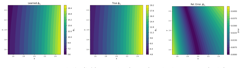
Summary. The paper proposes a kernel collocation method for approximating the principal Koopman eigenfunctions of a nonlinear system near a hyperbolic equilibrium. The eigenfunction is decomposed as φ_λ(x)=w^T x+h(x), where w is a left eigenvector of the linearization at the equilibrium and h solves the linear transport PDE (22) with boundary conditions h(x_e)=0 and ∇h(x_e)=0. The PDE is discretized by collocation and solved in a reproducing kernel Hilbert space via the representer formula (17)-(19). The paper claims rigorous error estimates: Theorem 5 asserts that the operator Dh=∇h·f−λh is a bounded bijection between Sobolev spaces on a bounded neighborhood Ω, yielding the stability bound (24), and Theorem 6 derives a fill-distance convergence rate from that bound. Numerical experiments in Sections 5.1–5.4 demonstrate recovery of known analytical eigenfunctions and level sets for the Duffing and gradient systems.
Significance. If Theorems 5 and 6 were valid, the paper would make a useful contribution: it would compute Koopman eigenfunctions without constructing the Koopman operator, with convergence guarantees and an explicit mechanism to avoid spectral pollution. The numerical demonstrations in Sections 5.1 and 5.2 show that the collocation approach can recover the nonlinear part h when the true eigenfunction is known. However, the advertised theoretical guarantees are the paper's central claim, and they are not established: the main well-posedness theorem is false as stated, and the convergence theorem depends on it. The numerical experiments are suggestive but do not compensate for the failure of the theoretical framework.
major comments (3)
- [Section 4, Theorem 5 (Eqs. (22)-(24))] The proof of Theorem 5 is invalid and its statement is false. Step 1 infers injectivity of D from hyperbolicity of the equilibrium, but hyperbolicity does not imply injectivity of a first-order transport operator on a bounded domain with only point constraints at the equilibrium. For the linear saddle f(x)=(-x1,x2), λ=-1, w=(1,0), and Ω=(-1,1)^2, the function h(x)=x1^3 x2^2 satisfies Dh=0, h(0)=0, and ∇h(0)=0, so ker(D) contains a nonzero smooth function. Step 2 invokes elliptic regularity for a first-order hyperbolic operator, which is not applicable. Consequently, the stability bound (24) and all results depending on the bounded invertibility of D, including Theorem 6, are not established.
- [Section 4, Theorem 6] The convergence estimate in Theorem 6 assumes that the exact solution h_λ lies in the RKHS H of the chosen kernel and that H embeds continuously into W^{m+1}_2(Ω). This is a strong regularity condition, analogous to analyticity for Gaussian kernels, and it is not verified or quantified anywhere in the paper. Moreover, the proof of Theorem 6 uses the stability bound (24) from Theorem 5, which is false as shown above. Thus the claimed convergence rate is not proven even under the additional RKHS assumptions.
- [Section 5, numerical experiments] The numerical experiments rely on hand-tuned kernel bandwidths σ1 and σ2 (Sections 5.1, 5.2, 5.3) and do not specify the regularization parameter η in Eq. (19), although Theorem 6 assumes η=0. The experiments only test cases with known analytical eigenfunctions; they cannot detect the failure of the well-posedness assumption on general bounded domains. The method may work on the particular examples, but the experiments do not substantiate the general theoretical claims made in Sections 4.
minor comments (5)
- [Section 3.2, Eq. (18)] The notation F(z_i)_j conflicts with the function space F introduced in Section 2.1; the vector field f should be used consistently throughout.
- [Section 3.1, Definition 4] The statement 'k spans H: H = span{k_x | x ∈ X}' should refer to the closure of the span, and the quantifier in item i should be 'for all x ∈ X' rather than 'for all x ∈ H'.
- [Section 4, Theorem 6] The theorem says the constants do not depend on λ or f, but the displayed bound contains the factor (∥f∥_{W^m_2(Ω,R^d)} + |λ|); this wording is misleading and should be clarified.
- [Section 2.2] The text uses 'principle eigenfunctions' instead of 'principal eigenfunctions'; the terminology should be unified.
- [Section 3.2, Eqs. (20)-(21)] The distributional pairings K(z, φ~) and K(φ~, φ~) involve products of the kernel with Dirac deltas and derivatives; the paper should specify the precise function-space setting in which these pairings are well defined for Gaussian kernels.
Circularity Check
No direct circularity: the core PDE-solving pipeline is self-contained, though the paper relies on self-citations to coauthor work and uses hand-tuned kernel bandwidths.
full rationale
The derivation chain is: (i) define Koopman eigenfunctions by ∂φ/∂x·f = λφ; (ii) decompose φ = wᵀx + h with w a left eigenvector of E = ∂f/∂x(0) and h the nonlinear part; (iii) substitute to obtain the linear PDE ∇h·f − λh = −wᵀG; (iv) solve this PDE by RKHS regression with the representer formula. None of these steps fits the target eigenfunction values or imports the conclusion as an input. The w and λ are obtained from the linearization and G from f, while the collocation constraints in (17) use only this known data, so the approximation is not circular by construction. The cited representer formula (Theorems 3–4, from Owhadi–Scovel, a coauthor text) is standard and is sketched in the paper itself, so the citation is not load-bearing in a circular sense; the decomposition 'following [26]' is elementary algebra verifiable from (8)–(11) within the paper. The main weaknesses are rigor issues, not circularity: Theorem 5's proof claims elliptic regularity and injectivity for the first-order transport operator D, which is mathematically unsupported and in fact false for simple linear saddles on bounded domains; Theorem 6 additionally assumes h_λ lies in the RKHS H, a strong smoothness condition. These are correctness concerns, not cases where a quantity is fitted and then renamed as a prediction. The hand-tuned bandwidths σ in Section 5 affect numerical accuracy but are not hidden fits of the eigenfunction values used as predictions. No circular step can be exhibited, so the score is low.
Assumptions & free parameters
free parameters (3)
- Gaussian kernel bandwidths σ1, σ2 =
σ1=σ2=2 (Ex5.1 λ1); σ1=2, σ2=3 (Ex5.1 λ2); σ1=σ2=3 (Ex5.2 λ1); σ1=σ2=7 (Ex5.2 λ2); σ1=σ2=15 (Ex5.3); σ=1.1 (Ex5.4)
- Regularization constant η =
not specified
- Number of collocation points and domain =
3600, 2500, 2500, 3379 over specified domains
assumptions (5)
- domain assumption The vector field f is C^m and the equilibrium is hyperbolic.
- domain assumption The principal eigenfunctions exist on the domain Ω and can be decomposed as w^T x + h(x).
- ad hoc to paper The operator D = ∇h·f - λh is a bounded bijection between W^{m+1}_2(Ω) and L_q(Ω).
- ad hoc to paper The true nonlinear part h_λ belongs to the RKHS H of the chosen kernel, and H embeds continuously into W^{m+1}_2(Ω).
- standard math Standard RKHS representer theorems and Sobolev embedding theorems.
Cite this review
Pith. "Pith review of Kernel Methods for the Approximation of the Eigenfunctions of the Koopman Operator." pith.science (2026). https://pith.science/paper/OIAWXAVM
@misc{pith2026241216588,
  author       = {Pith},
  title        = {Pith review of: Kernel Methods for the Approximation of the Eigenfunctions of the Koopman Operator},
  year         = {2026},
  howpublished = {\url{https://pith.science/paper/OIAWXAVM}},
  note         = {Machine review of arXiv:2412.16588}
}
read the original abstract
The Koopman operator provides a linear framework to study nonlinear dynamical systems. Its spectra offer valuable insights into system dynamics, but the operator can exhibit both discrete and continuous spectra, complicating direct computations. In this paper, we introduce a kernel-based method to construct the principal eigenfunctions of the Koopman operator without explicitly computing the operator itself. These principal eigenfunctions are associated with the equilibrium dynamics, and their eigenvalues match those of the linearization of the nonlinear system at the equilibrium point. We exploit the structure of the principal eigenfunctions by decomposing them into linear and nonlinear components. The linear part corresponds to the left eigenvector of the system's linearization at the equilibrium, while the nonlinear part is obtained by solving a partial differential equation (PDE) using kernel methods. Our approach avoids common issues such as spectral pollution and spurious eigenvalues, which can arise in previous methods. We demonstrate the effectiveness of our algorithm through numerical examples.
Figures


Figures from the paper (3 more)


Forward citations
Cited by 1 Pith paper
-
Koopman-Based Event-Triggered Control from Data
A data-driven event-triggered controller for discrete-time nonlinear systems is designed by lifting them into a higher-dimensional linear space via Koopman operators, with stability conditions posed as LMIs.
Reference graph
Works this paper leans on
-
[1]
H. Kantz and T. Schreiber, Nonlinear Time Series Analysis. USA: Cambridge University Press, 1997
work page 1997
-
[2]
Nonlinear prediction of chaotic time series,
M. Casdagli, “Nonlinear prediction of chaotic time series,” Physica D: Nonlinear Phenomena, vol. 35, no. 3, pp. 335 – 356, 1989. [Online]. Available: http://www.sciencedirect.com/science/article/pii/0167278989900742 16
arXiv 1989
-
[3]
J. L. Hudson, M. Kube, R. A. Adomaitis, I. G. Kevrekidis, A. S. Lapedes, and R. Farber, “Nonlinear signal processing and system identification: Applications to time series from electrochemical reactions,” Chemical Engineering Science, vol. 45, no. 8, pp. 2075–2081, 1990. [Online]. Available: https://www.sciencedirect.com/science/article/pii/000925099080079T
arXiv 1990
-
[4]
Discrete-vs. continuous-time nonlinear signal processing of cu electrodissolu- tion data,
R. Rico-Martinez, K. Krischer, I. Kevrekidis, M. Kube, and J. Hudson, “Discrete-vs. continuous-time nonlinear signal processing of cu electrodissolu- tion data,” Chemical Engineering Communications, vol. 118, no. 1, pp. 25–48, 1992
work page 1992
-
[5]
Nonlinear system identification using neural networks: dy- namics and instabilities,
O. Grandstrand, “Nonlinear system identification using neural networks: dy- namics and instabilities,” in Neural Networks for Chemical Engineers , A. B. Bulsari, Ed. Elsevier: Elsevier, 1995, ch. 16, pp. 409–442
work page 1995
-
[6]
Identification of distributed parameter systems: A neural net based approach,
R. Gonz´ alez-Garc ´ ıa, R. Rico-Mart ´ ınez, and I. Kevrekidis, “Identification of distributed parameter systems: A neural net based approach,” Computers and Chemical Engineering , vol. 22, pp. S965–S968, 1998, european Symposium on Computer Aided Process Engineering-8. [Online]. Available: https://www.sciencedirect.com/science/article/pii/S0098135498001914
work page 1998
-
[7]
A. Chattopadhyay, P. Hassanzadeh, K. V. Palem, and D. Subramanian, “Data-driven prediction of a multi-scale lorenz 96 chaotic system using a hierarchy of deep learning methods: Reservoir computing, ann, and RNN-LSTM,” CoRR, vol. abs/1906.08829, 2019. [Online]. Available: http://arxiv.org/abs/1906.08829
work page Pith review arXiv 1906
-
[8]
Discovering governing equations from data by sparse identification of nonlinear dynamical systems,
S. L. Brunton, J. L. Proctor, and J. N. Kutz, “Discovering governing equations from data by sparse identification of nonlinear dynamical systems,” Proceedings of the National Academy of Sciences , vol. 113, no. 15, pp. 3932–3937, 2016. [Online]. Available: https://www.pnas.org/content/113/15/3932
work page 2016
Show all 66 references
-
[9]
Using machine learning to replicate chaotic attractors and calculate lyapunov exponents from data,
J. Pathak, Z. Lu, B. R. Hunt, M. Girvan, and E. Ott, “Using machine learning to replicate chaotic attractors and calculate lyapunov exponents from data,” Chaos: An Interdisciplinary Journal of Nonlinear Science , vol. 27, no. 12, p. 121102, 2017. [Online]. Available: https://d...
2017 doi
-
[10]
Nielsen, Practical Time Series Analysis: Prediction with Statistics and Ma- chine Learning
A. Nielsen, Practical Time Series Analysis: Prediction with Statistics and Ma- chine Learning. O’Reilly Media, 2019
2019
-
[11]
Abarbanel, Analysis of Observed Chaotic Data , ser
H. Abarbanel, Analysis of Observed Chaotic Data , ser. Institute for Nonlinear Science. Springer New York, 2012
2012
-
[12]
A New Kernel-Based Approach for NonlinearSystem Identification,
G. Pillonetto, M. H. Quang, and A. Chiuso, “A New Kernel-Based Approach for NonlinearSystem Identification,” IEEE Transactions on Automatic Control, vol. 56, no. 12, pp. 2825–2840, Dec. 2011. 17
2011
-
[13]
Predicting Catastrophes in Nonlinear Dynamical Systems by Compressive Sensing,
W.-X. Wang, R. Yang, Y.-C. Lai, V. Kovanis, and C. Grebogi, “Predicting Catastrophes in Nonlinear Dynamical Systems by Compressive Sensing,” Phys- ical Review Letters, vol. 106, no. 15, p. 154101, Apr. 2011
2011
-
[14]
Discovering governing equations from data by sparse identification of nonlinear dynamical systems,
S. L. Brunton, J. L. Proctor, and J. N. Kutz, “Discovering governing equations from data by sparse identification of nonlinear dynamical systems,” Proceedings of the National Academy of Sciences , vol. 113, no. 15, pp. 3932–3937, 2016
2016
-
[15]
Deep learning for universal linear embeddings of nonlinear dynamics,
B. Lusch, J. N. Kutz, and S. L. Brunton, “Deep learning for universal linear embeddings of nonlinear dynamics,” Nature Communications, vol. 9, no. 1, p. 4950, Dec. 2018
2018
-
[16]
Learning dominant physical processes with data-driven balance models,
J. L. Callaham, J. V. Koch, B. W. Brunton, J. N. Kutz, and S. L. Brunton, “Learning dominant physical processes with data-driven balance models,” Na- ture Communications, vol. 12, no. 1, p. 1016, Dec. 2021
2021
-
[17]
Physics-constrained, low-dimensional models for magnetohydrodynamics: First-principles and data-driven approaches,
A. A. Kaptanoglu, K. D. Morgan, C. J. Hansen, and S. L. Brunton, “Physics-constrained, low-dimensional models for magnetohydrodynamics: First-principles and data-driven approaches,”Physical Review E, vol. 104, no. 1, p. 015206, Jul. 2021
2021
-
[18]
Parsimony as the ultimate regularizer for physics-informed machine learning,
J. N. Kutz and S. L. Brunton, “Parsimony as the ultimate regularizer for physics-informed machine learning,” Nonlinear Dynamics, Jan. 2022
2022
-
[19]
Dynamical systems of continuous spec- tra,
B. O. Koopman and J. v. Neumann, “Dynamical systems of continuous spec- tra,” Proceedings of the National Academy of Sciences , vol. 18, no. 3, pp. 255– 263, 1932
1932
-
[20]
Spectral properties of dynamical systems, model reduction and de- compositions,
I. Mezi´ c, “Spectral properties of dynamical systems, model reduction and de- compositions,” Nonlinear Dynamics, vol. 41, no. 1, pp. 309–325, 2005
2005
-
[21]
Global stability analysis using the eigenfunctions of the koopman operator,
A. Mauroy and I. Mezi´ c, “Global stability analysis using the eigenfunctions of the koopman operator,” IEEE Transactions on Automatic Control , vol. 61, no. 11, pp. 3356–3369, 2016
2016
-
[22]
Spectral koopman method for identifying stability boundary,
B. Umathe and U. Vaidya, “Spectral koopman method for identifying stability boundary,” IEEE Control Systems Letters , 2023
2023
-
[23]
Data-driven transient stability analysis using the koopman operator,
A. R. Matavalam, B. Hou, H. Choi, S. Bose, and U. Vaidya, “Data-driven transient stability analysis using the koopman operator,” International Journal of Electrical Power & Energy Systems , vol. 162, p. 110307, 2024
2024
-
[24]
Spectral analysis of koopman operator and nonlinear optimal con- trol,
U. Vaidya, “Spectral analysis of koopman operator and nonlinear optimal con- trol,” in 2022 IEEE 61st Conference on Decision and Control (CDC) . IEEE, 2022, pp. 3853–3858
2022
-
[25]
When Koopman meets Hamilton and Jacobi,
——, “When Koopman meets Hamilton and Jacobi,” In preprint, 2024. 18
2024
-
[26]
Path-integral formula for com- puting koopman eigenfunctions,
S. A. Deka, S. S. Narayanan, and U. Vaidya, “Path-integral formula for com- puting koopman eigenfunctions,” in 2023 62nd IEEE Conference on Decision and Control (CDC) . IEEE, 2023, pp. 6641–6646
2023
-
[27]
The foundations of infinite-dimensional spectral computations,
M. Colbrook, “The foundations of infinite-dimensional spectral computations,” Ph.D. dissertation, University of Cambridge, 2020
2020
-
[28]
A data–driven approx- imation of the koopman operator: Extending dynamic mode decomposition,
M. O. Williams, I. G. Kevrekidis, and C. W. Rowley, “A data–driven approx- imation of the koopman operator: Extending dynamic mode decomposition,” Journal of Nonlinear Science , vol. 25, no. 6, pp. 1307–1346, 2015
2015
-
[29]
Data- driven approximation of the Koopman generator: Model reduction, system identification, and control,
S. Klus, F. N¨ uske, S. Peitz, J.-H. Niemann, C. Clementi, and C. Sch¨ utte, “Data- driven approximation of the Koopman generator: Model reduction, system identification, and control,” Physica D: Nonlinear Phenomena , vol. 406, p. 132416, 2020
2020
-
[30]
Data-driven koopman op- erators for model reduction and control of systems with symmetries,
B. Peherstorfer, S. L. Brunton, and J. N. Kutz, “Data-driven koopman op- erators for model reduction and control of systems with symmetries,” SIAM Journal on Applied Dynamical Systems , vol. 19, no. 3, pp. 1894–1920, 2020
1920
-
[31]
Kernel-based dynamic mode decomposition,
S. Klus, F. N¨ uske, P. Koltai, I. G. Kevrekidis, C. Sch¨ utte, and C. Clementi, “Kernel-based dynamic mode decomposition,” Journal of Computational Dy- namics, vol. 2, no. 2, pp. 247–265, 2015
2015
-
[32]
Koopman spectra in reproducing kernel hilbert spaces,
S. Das and D. Giannakis, “Koopman spectra in reproducing kernel hilbert spaces,” Applied and Computational Harmonic Analysis , vol. 49, no. 2, pp. 573–607, 2020. [Online]. Available: https://www.sciencedirect.com/science/ article/pii/S1063520320300427
2020
-
[33]
Sparse learning of dynamical systems in RKHS: An operator-theoretic approach,
B. Hou, S. Sanjari, N. Dahlin, S. Bose, and U. Vaidya, “Sparse learning of dynamical systems in RKHS: An operator-theoretic approach,” inInternational Conference on Machine Learning . PMLR, 2023, pp. 13 325–13 352
2023
-
[34]
Koopman operators with intrinsic observables in rigged reproducing kernel hilbert spaces,
I. Ishikawa, Y. Hashimoto, M. Ikeda, and Y. Kawahara, “Koopman operators with intrinsic observables in rigged reproducing kernel hilbert spaces,” 2024. [Online]. Available: https://arxiv.org/abs/2403.02524
2024
-
[35]
On the mathematical foundations of learning,
F. Cucker and S. Smale, “On the mathematical foundations of learning,” Bul- letin of the American mathematical society , vol. 39, no. 1, pp. 1–49, 2002
2002
-
[36]
Solving and learning nonlinear pdes with gaussian processes,
Y. Chen, B. Hosseini, H. Owhadi, and A. M. Stuart, “Solving and learning nonlinear pdes with gaussian processes,” Journal of Computational Physics , vol. 447, 2021
2021
-
[37]
Error analysis of kernel/gp methods for nonlinear and parametric pdes,
P. Batlle, Y. Chen, B. Hosseini, H. Owhadi, and A. M. Stuart, “Error analysis of kernel/gp methods for nonlinear and parametric pdes,” Journal of Compu- tational Physics , vol. 520, p. 113488, 2025. 19
2025
-
[38]
Computational Graph Completion,
H. Owhadi, “Computational Graph Completion,” Research in the Mathematical Sciences, vol. 9(2), no. 27, 2021. [Online]. Available: https://arxiv.org/abs/ 2110.10323
2021 arXiv
-
[39]
Codiscovering graphical structure and functional relationships within data: A gaussian process framework for connecting the dots,
T. Bourdais, P. Batlle, X. Yang, R. Baptista, N. Rouquette, and H. Owhadi, “Codiscovering graphical structure and functional relationships within data: A gaussian process framework for connecting the dots,” Proceedings of the Na- tional Academy of Sciences , vol. 121, no. 32, ...
2024
-
[40]
Greedy kernel methods for center manifold approximation,
B. Haasdonk, B. Hamzi, G. Santin, and D. Wittwar, “Greedy kernel methods for center manifold approximation,” Proc. of ICOSAHOM 2018, International Conference on Spectral and High Order Methods , vol. 427, no. 1, 2018, https: //arxiv.org/abs/1810.11329
2018 arXiv
-
[41]
Kernel methods for center manifold approximation and a weak data- based version of the center manifold theorems,
——, “Kernel methods for center manifold approximation and a weak data- based version of the center manifold theorems,” Physica D, 2021
2021
-
[42]
Approximation of Lya- punov functions from noisy data,
P. Giesl, B. Hamzi, M. Rasmussen, and K. Webster, “Approximation of Lya- punov functions from noisy data,” Journal of Computational Dynamics , vol. 7, pp. 57–81, 2019, https://arxiv.org/abs/1601.01568
2019 arXiv
-
[43]
Learning dynamical systems from data: A simple cross-validation perspective, Part I: Parametric Kernel Flows,
B. Hamzi and H. Owhadi, “Learning dynamical systems from data: A simple cross-validation perspective, Part I: Parametric Kernel Flows,” Physica D: Nonlinear Phenomena , vol. 421, p. 132817, 2021. [Online]. Available: https://www.sciencedirect.com/science/article/pii/S0167278920308186
2021
-
[44]
Kernel methods for the approximation of discrete- time linear autonomous and control systems,
B. Hamzi and F. Colonius, “Kernel methods for the approximation of discrete- time linear autonomous and control systems,” SN Applied Sciences , vol. 1, no. 7, pp. 1–12, 2019
2019
-
[45]
Kernel-based approximation of the Koopman generator and Schr¨ odinger operator,
S. Klus, F. Nuske, and B. Hamzi, “Kernel-based approximation of the Koopman generator and Schr¨ odinger operator,” Entropy, vol. 22, 2020, https://www. mdpi.com/1099-4300/22/7/722
2020
-
[46]
Operator-theoretic framework for forecasting nonlinear time series with kernel analog techniques,
R. Alexander and D. Giannakis, “Operator-theoretic framework for forecasting nonlinear time series with kernel analog techniques,” Physica D: Nonlinear Phenomena , vol. 409, p. 132520, 2020. [Online]. Available: http://www.sciencedirect.com/science/article/pii/S016727891930377X
2020
-
[47]
Dimensionality reduction of complex metastable systems via kernel embeddings of transition manifold,
A. B. S. K. B. H. P. Koltai, and C. Schutte, “Dimensionality reduction of complex metastable systems via kernel embeddings of transition manifold,” Journal of Nonlinear Science , vol. 31(3), 2019
2019
-
[49]
Kernel methods for the approximation of nonlinear systems,
——, “Kernel methods for the approximation of nonlinear systems,” SIAM J. Control and Optimization , 2017, https://arxiv.org/abs/1108.2903
2017 arXiv
-
[50]
Kernel methods for the approximation of some key quantities of non- linear systems,
——, “Kernel methods for the approximation of some key quantities of non- linear systems,” Journal of Computational Dynamics , vol. 1, 2017, http: //arxiv.org/abs/1204.0563
2017 arXiv
-
[51]
A note on kernel methods for multiscale systems with critical transitions,
B. Hamzi, C. Kuehn, and S. Mohamed, “A note on kernel methods for multiscale systems with critical transitions,” Mathematical Methods in the Applied Sciences , vol. 42, no. 3, pp. 907–917, 2019. [Online]. Available: https://onlinelibrary.wiley.com/doi/abs/10.1002/mma.5394
2019 doi
-
[52]
Learning dynamical systems from data: A simple cross-validation perspective, Part V: Sparse Kernel Flows for 132 chaotic dynamical systems,
L. Yang, X. Sun, B. Hamzi, H. Owhadi, and N. Xie, “Learning dynamical systems from data: A simple cross-validation perspective, Part V: Sparse Kernel Flows for 132 chaotic dynamical systems,” Physica D, vol. 460, 2022
2022
-
[53]
Learning dynamical systems from data: A simple cross-validation perspective, Part VI: Hausdorff-metric based Kernel Flows to learn Attractors and Invariant Sets,
L. Yang, B. Hamzi, Y. Kevrekidis, H. Owhadi, X. Sun, and N. Xie, “Learning dynamical systems from data: A simple cross-validation perspective, Part VI: Hausdorff-metric based Kernel Flows to learn Attractors and Invariant Sets,” Physica D, 2023
2023
-
[54]
Propagating uncer- tainty through system dynamics in reproducing kernel hilbert space,
B. Hou, A. R. R. Matavalam, S. Bose, and U. Vaidya, “Propagating uncer- tainty through system dynamics in reproducing kernel hilbert space,” Physica D: Nonlinear Phenomena , p. 134168, 2024
2024
-
[55]
Gaussian processes simplify differential equations,
J. Lee, B. Hamzi, Y. Kevrekidis, and H. Owhadi, “Gaussian processes simplify differential equations,” September 2024. [Online]. Available: https://www.researchgate.net/publication/383680496 Gaussian Processes Simplify Differential Equations
2024
-
[56]
Kernel sum of squares for data adapted kernel learning of dynamical systems from data: A global optimization approach,
D. Lengyel, B. Hamzi, H. Owhadi, and P. Parpas, “Kernel sum of squares for data adapted kernel learning of dynamical systems from data: A global optimization approach,” arXiv preprint arXiv:2408.06465 , 2024. [Online]. Available: https://www.arxiv.org/pdf/2408.06465
2024 arXiv
-
[57]
Kernel methods for surrogate modeling,
G. Santin and B. Haasdonk, “Kernel methods for surrogate modeling,” System and Data-Driven Methods and Algorithms , 2019, https://arxiv.org/abs/1907. 105566
2019
-
[58]
Limits and powers of koopman learning,
M. J. Colbrook, I. Mezi´ c, and A. Stepanenko, “Limits and powers of koopman learning,” arXiv preprint arXiv:2407.06312 , 2024
2024 arXiv
-
[59]
Koopman kernel regression,
P. Bevanda, M. Beier, A. Lederer, S. Sosnowski, E. H¨ ullermeier, and S. Hirche, “Koopman kernel regression,” Advances in Neural Information Processing Sys- tems, vol. 36, 2024. 21
2024
-
[60]
Spectrum of the koopman operator, spectral expansions in functional spaces, and state-space geometry,
I. Mezi´ c, “Spectrum of the koopman operator, spectral expansions in functional spaces, and state-space geometry,” Journal of Nonlinear Science, vol. 30, no. 5, pp. 2091–2145, 2020
2020
-
[61]
Koopman operator, geometry, and learning of dynamical systems,
——, “Koopman operator, geometry, and learning of dynamical systems,” Not. Am. Math. Soc. , vol. 68, no. 7, pp. 1087–1105, 2021
2021
-
[62]
Lasota and M
A. Lasota and M. C. Mackey, Chaos, Fractals, and Noise: Stochastic Aspects of Dynamics . New York: Springer-Verlag, 1994
1994
-
[63]
Applied koopmanism,
M. Budiˇ si´ c, R. Mohr, and I. Mezi´ c, “Applied koopmanism,”Chaos: An Inter- disciplinary Journal of Nonlinear Science , vol. 22, no. 4, p. 047510, 2012
2012
-
[64]
Arnold, Geometrical Methods in the Theory of Ordinary Differential Equa- tions
V. Arnold, Geometrical Methods in the Theory of Ordinary Differential Equa- tions. Springer Verlag, 2012
2012
-
[65]
Theory of reproducing kernels,
N. Aronszajn, “Theory of reproducing kernels,” Transactions of the American Mathematical Society, vol. 68, no. 3, pp. 337–404, 1950. [Online]. Available: http://dx.doi.org/10.2307/1990404
1950 doi
-
[66]
Owhadi and C
H. Owhadi and C. Scovel, Operator-Adapted Wavelets, Fast Solvers and Nu- merical Homogenization: From a Game Theoretic Approach to Numerical Ap- proximation and Algorithm Design . Cambridge Monographs on Applied and Computational Mathematics. Cambridge University Press, 2019
2019
-
[67]
Sobolev bounds on functions with scattered zeros, with applications to radial basis function surface fitting,
F. J. Narcowich, J. D. Ward, and H. Wendland, “Sobolev bounds on functions with scattered zeros, with applications to radial basis function surface fitting,” Mathematics of Computation , vol. 74, no. 250, pp. 743–763, 2005. 22
2005
Reviewed August 11, 2026 · model on record in the stance chip above.
Discussion (0). Continue with ORCID to comment.