REVIEW 3 major objections 6 minor 3 cited by
Optimal Response for Hyperbolic Systems by the fast adjoint response method
T0 review · 3 major / 6 minor · reviewed 2026-08-10 · deepseek-v4-flash
Pith's one-line read A unique optimal perturbation exists for hyperbolic systems, and its Fourier coefficients are linear responses of a basis.
desk verdict First general optimal-response result for hyperbolic systems, with a genuinely high-dimensional numerical demonstration; the abstract overreaches by omitting boundedness, but the core result is sound and worth refereeing. read the letter →
The pith
A machine-rendered reading of the paper's core claim, the machinery that carries it, and where it could break.
The reading
What carries the argument
The fast adjoint response formula, Eq. (6), $$R(X) = \lim_{W\to\infty} \mu\!\left[ \big(S(d\Phi) + \varphi_W\, S(\operatorname{div}_v f_*)\big) X + \varphi_W\, \operatorname{div}_v X \right],$$ combines the adjoint shadowing operator $S$ (whose fixed-point equation is $\omega = f^*\omega + d\Phi$) with the equivariant divergence formula $\operatorname{div}_v X = \tilde\varepsilon \nabla_{\tilde e} X$. Because every term is a pointwise function on the attractor, this formula converts response estimates into decay-of-correlation estimates, which is what yields the $C^{1,\alpha}$ bound in Lemma 1 and ultimately the Hilbert-space representative $v$ via Riesz representation.
What would settle it
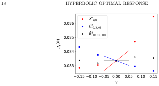
For one of the toral examples, compute $\mu_\gamma(\Phi)$ for several small $\gamma$ by direct long-orbit averages for a perturbation $X$, fit the slope at $\gamma=0$, and compare it with $R(X)$ from the fast adjoint formula; a systematic mismatch beyond the stated sampling error would falsify the representation (6) and hence the computed $v$.
Extended reading notes
Core claim
The paper's central claim is that the optimal response problem for a uniformly hyperbolic (Axiom A) system has a unique solution under natural convexity assumptions, and that the solution is given explicitly by the Riesz representative of the linear response operator. Lemma 1 shows that the response operator $R$ extends to $C^{1,\alpha}$ and satisfies $|R(X)| \le C\|X\|_{C^{1,\alpha}}$, so $R$ is a continuous linear functional on any Hilbert space $H$ continuously embedded in $C^3$. Riesz representation then yields a unique $v\in H$ with $R(w)=\langle w,v\rangle_H$; when the feasible set is the unit ball, the unique maximizer is $X_{\mathrm{opt}} = v/\|v\|_H$, and its Fourier coefficients are $c_i = R(b_i)$ for an orthonormal basis $\{b_i\}$. The same conclusion holds both for perturbations by composition with a diffeomorphism near the identity and for additive perturbations of the map, and the paper verifies the construction numerically on 2-, 3-, and 21-dimensional toral examples.
Load-bearing premise
The load-bearing premise is that the fast adjoint response formula exactly represents the linear response of the unperturbed Axiom A system, which requires exponential decay of correlations; for the numerical examples, the required uniform hyperbolicity is asserted rather than rigorously verified.
Editorial extensions
If this is right
- When the feasible set is the unit ball of $H$, the unique optimal perturbation is $v/\|v\|_H$, so computing the optimizer reduces to computing the linear response of each basis element, $c_i = R(b_i)$.
- The same statement holds for two perturbation mechanisms: composing the map with a diffeomorphism near the identity, and adding a deterministic perturbation to the map, with the additive case represented by $I(X') = X'\circ f^{-1}$.
- For any strictly convex, bounded, closed feasible set with a nonzero response functional, the optimal perturbation exists and is unique, extending the unit-ball result to constrained control sets such as perturbations acting only on selected coordinates.
- On the torus, the Fourier expansion of $v$ is explicitly constructed from trigonometric basis functions, and on more general manifolds $v$ solves a high-order Laplacian equation with boundary conditions given in Section 6.
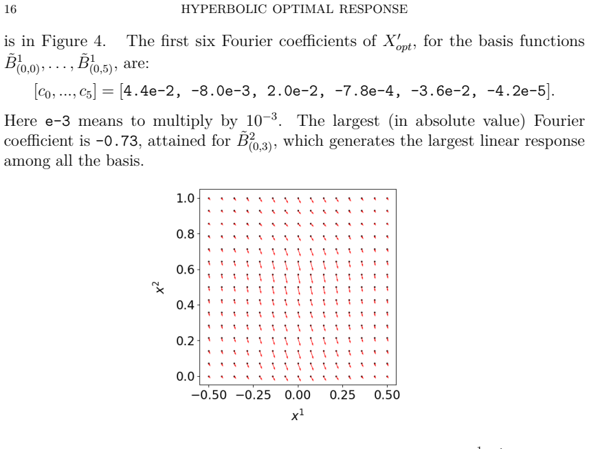
- The numerical experiments in dimensions 2, 3, and 21 confirm that the computed optimal perturbation produces a larger linear response than every single basis element and matches the finite-difference trend of $\mu_\gamma(\Phi)$.
Reading between the lines
- The paper leaves open whether the linear response itself exists for perturbations that are only $C^{1,\alpha}$; if it does, the $C^{1,\alpha}$ bound in Lemma 1 suggests the optimizer could be defined over rougher perturbation classes than $C^3$, but this requires a separate proof.
- Because each coefficient $c_i = R(b_i)$ is an independent orbit-based computation, the method is embarrassingly parallel; the reported wall-clock times suggest that with enough cores the 21-dimensional example could be pushed to much larger basis sets.
- The cost of the Fourier approach grows with the number of basis functions, not with the phase-space dimension, so choosing a deliberately small Hilbert space $H$ (e.g., perturbations depending only on one coordinate) is a natural route to control high-dimensional systems, as the 21-dimensional example illustrates.
- For applied settings with a prescribed family of controls, the strict-convexity result means the optimal infinitesimal control is unique; testing whether that uniqueness survives finite-time or nonlinear effects would be a natural next step.
Signed reviews
Editorial analysis
A structured set of objections, weighed in public.
Referee Report
Summary. The paper studies the optimal linear response problem for uniformly hyperbolic (mixing Axiom A) diffeomorphisms. Given an observable and a convex feasible set P of infinitesimal perturbations contained in a Hilbert space H continuously embedded into C^3 vector fields, it seeks the perturbation maximizing the linear response R. Using the authors' fast adjoint response formula, Lemma 1 establishes a bound on R in the C^{1,α} norm, and Section 4.1 gives existence and uniqueness for bounded strictly convex closed feasible sets. When P is the unit ball, the optimizer is identified with the normalized Riesz representative v of R, and Section 4.3 expands v in a Fourier basis on tori. Section 5 implements the algorithm on 2-, 3-, and 21-dimensional solenoid-like maps, validating the computed optimal response against finite-difference estimates of the perturbed measure. Section 6 sketches a PDE-based approach for manifolds with boundary.
Significance. If the main estimates are correct, the paper offers a general Hilbert-space framework for optimal linear response in hyperbolic systems and a practical adjoint-based algorithm that scales favorably when the feasible perturbation set is small relative to the phase-space dimension. The numerical coefficients are computed, not fitted, and the validation against direct finite-difference approximations of μ_γ(Φ) is an external check. The main theorem in Proposition 3 is defensible once boundedness is included; the issues identified below are local to the statements and definitions, not to the central numerical strategy.
major comments (3)
- [Abstract; §4.1, Proposition 3] The uniqueness theorem as advertised is false because boundedness of P is omitted. For example, take H=R^2 and P={(x,y): y≥x^2}, which is closed, convex, strictly convex, and unbounded; the continuous linear functional L(x,y)=y is unbounded above on P, so no maximizer exists. This example can be embedded in the paper's setting by mapping (x,y) to the constant vector field yV for a nonzero V∈C^3 and choosing an observable with R(V)≠0. Proposition 3 correctly assumes P is bounded; the abstract and the informal statement in Section 1.2 must also state boundedness of P, together with the condition that R is not identically zero on P. The unit-ball applications are unaffected by this correction, but the advertised central claim overreaches as written.
- [Definition 1] Definition 1 as written requires γx+(1−γ)y∈int(A) for all pairs x,y∈A, including x=y. For x=y the condition forces every point of A to be interior, so no closed convex set with nonempty boundary, including the unit ball which the text explicitly says is strictly convex, satisfies the definition. The intended definition must be for all x≠y. Proposition 3's uniqueness conclusion relies on this corrected reading.
- [Proposition 4] The statement of Proposition 4 omits the hypothesis that P is the unit ball of H. As written it is applied to the general optimization problem (11) over an arbitrary bounded strictly convex closed set, but the formula X_opt=v/||v||_H is only correct for the unit ball; for a ball of radius r the maximizer is r v/||v||_H. The preceding paragraph indicates the intended setting, but the proposition itself should state explicitly that P is the unit ball.
minor comments (6)
- [Lemma 1] The statement writes |R(X)|≤ C||X||_{C^{1,α}}≤||X||_{C^3}; the second inequality is not generally true with constant 1 and should read ||X||_{C^{1,α}}≤ C||X||_{C^3} (or the C^3 norm should be defined to dominate the C^{1,α} norm by construction).
- [Proof of Lemma 1, estimate for R_2W] The estimate writes a sum of C λ^n for n from −W to W; for negative n this should be C λ^{|n|}, otherwise the summand grows as n becomes negative.
- [Proposition 3] Proposition 3 refers to 'problem (20)', but at that point the relevant problem is (11); the reference should be corrected.
- [§5.1 and §5.2] The feasible set is written as P:={||X'||_{H^5}=1}, which is the unit sphere rather than the unit ball used in Propositions 5 and 6. For a linear objective the maximizer is the same, but the feasible set should be written consistently with the theoretical statement.
- [§5.1–5.3] The three maps are described as 'solenoid-like' and asserted to be hyperbolic, but no verification of uniform hyperbolicity or exponential decay of correlations is given. Since Lemma 1 and the fast adjoint response formula assume such a regime, the numerical claims should either include a check of hyperbolicity or be phrased as illustrative computations whose theoretical guarantees require the stated hypotheses.
- [§4.3] The text says 'M = TM is the M dimensional torus'; this should be M = T^M (or the notation should be introduced consistently).
Circularity Check
No circularity: the response coefficients are computed, not fitted, and the self-cited fast adjoint formula is independently published prior work.
full rationale
The derivation is self-contained in the relevant sense. The linear response operator R is defined as the derivative of the physical-measure expectation (Eq. (6)), and its boundedness on C^{1,alpha} is proved in Lemma 1 using the fast adjoint response formula, which is a previously published theorem from [20,22] with stated assumptions (uniform hyperbolicity, decay of correlations) that do not include the target result. The optimal perturbation is obtained by the Riesz representation theorem and computed from Fourier coefficients c_i = R(b_i) (Proposition 4); these coefficients are computed by applying the response operator to basis elements rather than fitted to the quantity being predicted. The numerical verification compares the computed linear response with independently simulated finite-difference slopes mu_gamma(Phi), so the comparisons are external to the fitted values. The only manuscript-level caveat, unrelated to circularity, is that the abstract states existence and uniqueness for a strictly convex closed P without boundedness, while the proof (Proposition 3) explicitly assumes P is bounded; this is an overstatement and a correctness issue, not a circular reduction. Because no key claim reduces to its own inputs by construction or through a load-bearing self-citation, the circularity score is 0.
Assumptions & free parameters
free parameters (3)
- Sobolev norm weights C_0,...,C_p in H^p inner product =
C_l = (2*pi)^(-2l) in numerical examples
- Sobolev index p of feasible space H^p =
p=5 in 2d/3d examples, p=4 in 21d example
- Numerical truncation and algorithm parameters N, W, Nseg, A =
N=15 (2d), 11 (3d), 21 (21d); W=10; Nseg=20; A=4000
assumptions (7)
- domain assumption The system (M,f) is a C^3 diffeomorphism with a mixing Axiom A attractor K and physical measure mu with exponential decay of correlations for Holder observables.
- domain assumption The fast adjoint response formula (Eq. (6)) from [20,22] correctly represents the linear response for C^3 perturbations.
- standard math Ruelle's linear response theorem for C^3 perturbations of uniformly hyperbolic systems.
- standard math Sobolev embedding H^p subset C^3 for p >= 4 + floor(M/2).
- standard math Riesz representation theorem in Hilbert spaces.
- standard math Closed bounded convex sets in Hilbert space are weakly compact, so continuous linear functionals attain maxima.
- standard math Composition with the C^3 inverse diffeomorphism f^{-1} preserves Sobolev regularity H^p.
Cite this review
Pith. "Pith review of Optimal Response for Hyperbolic Systems by the fast adjoint response method." pith.science (2026). https://pith.science/paper/SW4NOG7I
@misc{pith2026250102395,
  author       = {Pith},
  title        = {Pith review of: Optimal Response for Hyperbolic Systems by the fast adjoint response method},
  year         = {2026},
  howpublished = {\url{https://pith.science/paper/SW4NOG7I}},
  note         = {Machine review of arXiv:2501.02395}
}
abstract
In a uniformly hyperbolic system, we consider the problem of finding the optimal infinitesimal perturbation to apply to the system, from a certain set $P$ of feasible ones, to maximally increase the expectation of a given observation function. We perturb the system both by composing with a diffeomorphism near the identity or by adding a deterministic perturbation to the dynamics. In both cases, using the fast adjoint response formula, we show that the linear response operator, which associates the response of the expectation to the perturbation on the dynamics, is bounded in terms of the $C^{1,\alpha}$ norm of the perturbation. Under the assumption that $P$ is a strictly convex, closed subset of a Hilbert space $\cH$ that can be continuously mapped in the space of $C^3$ vector fields on our phase space, we show that there is a unique optimal perturbation in $P$ that maximizes the increase of the given observation function. Furthermore since the response operator is represented by a certain element $v$ of $\cH$, when the feasible set $P$ is the unit ball of $\cH$, the optimal perturbation is $v/||v||_{\cH}$. We also show how to compute the Fourier expansion $v$ in different cases. Our approach can work even on high dimensional systems. We demonstrate our method on numerical examples in dimensions 2, 3, and 21.
Figures


Figures from the paper (7 more)




Forward citations
Cited by 3 Pith papers
-
Markov matrix perturbations to optimize dynamical and entropy functionals
Linear-response optimization algorithms are derived for entropy, KL divergence, and entropy production on Markov chains, with a drift-reconstruction protocol linking matrix perturbations to vector field forcing.
-
Divergence-Kernel method for scores of random systems
New divergence-kernel formulas compute scores of SDEs with multiplicative noise via pathwise Monte Carlo, without hyperbolicity assumptions.
-
Optimal response for stochastic differential equations by local kernel perturbations
For SDEs on R^d, the paper proves existence and uniqueness of the optimal infinitesimal local kernel perturbation maximizing the linear response of an observable, and demonstrates a numerical approximation on a double...
Reference graph
Works this paper leans on
- [1]
- [2]
-
[3]
W. Bahsoun, S. Galatolo, I. Nisoli, and X. Niu. A rigorous computational approach to linear response. Nonlinearity, 31:1073–1109, 2018
work page 2018
-
[4]
V. Baladi. Linear response, or else. Proceedings of the International Congress of Mathematicians Seoul 2014, pages 525–545, 2014. 24 HYPERBOLIC OPTIMAL RESPONSE
work page 2014
- [5]
-
[6]
N. Chandramoorthy and M. Jézéquel. Rigorous justification for the space-split sensitivity algorithm to compute linear response in Anosov systems.arxiv:2109.02750, pages 1–33, 2021
work page Pith review arXiv 2021
-
[7]
M. F. Demers, N. Kiamari, and C. Liverani.Transfer operators in hyperbolic dynamics. An introduction. Colloquio Brasilero de Matematica. IMPA, 2021
work page 2021
-
[8]
L. C. Evans. Partial Differential Equations: Second Edition, volume 19. AMS, Graduate Studies in Mathematics, 2010
work page 2010
Show all 27 references
-
[9]
Froyland
G. Froyland. On Ulam approximation of the isolated spectrum and eigenfunctions of hyperbolic maps. Discrete and Continuous Dynamical Systems, 17:671–689, 2007
2007
-
[10]
Froyland and S
G. Froyland and S. Galatolo. Optimal linear response for expanding circle maps. https://arxiv.org/abs/2310.19191, 10 2023
2023 arXiv
-
[11]
Galatolo
S. Galatolo. Self-consistent transfer operators: Invariant measures, convergence to equilibrium, linear response and control of the statistical properties.Communications in Mathematical Physics, 395:715–772, 10 2022
2022
-
[12]
Galatolo and P
S. Galatolo and P. Giulietti. A linear response for dynamical systems with additive noise. Nonlinearity, 32:2269–2301, 6 2019
2019
-
[13]
Galatolo and M
S. Galatolo and M. Pollicott. Controlling the statistical properties of expanding maps. Nonlinearity, 30:2737–2751, 7 2017
2017
-
[14]
Ghil and V
M. Ghil and V. Lucarini. The physics of climate variability and climate change.Reviews of Modern Physics, 92:035002, 7 2020
2020
-
[15]
Gouëzel and C
S. Gouëzel and C. Liverani. Banach spaces adapted to Anosov systems.Ergodic Theory and Dynamical Systems, 26:189–217, 2006
2006
-
[16]
Kloeckner
B. Kloeckner. The linear request problem.Proceedings of the American Mathematical Society, 146:2953–2962, 3 2018
2018
-
[17]
R. S. MacKay. Management of complex dynamical systems.Nonlinearity, 31:R52–R65, 2 2018
2018
-
[18]
A. Ni. Fast differentiation of chaos on an orbit.arXiv:2009.00595, pages 1–28, 2020
2009
-
[19]
A. Ni. Fast adjoint algorithm for linear responses of hyperbolic chaos.SIAM Journal on Applied Dynamical Systems, 22:2792–2824, 12 2023
2023
-
[20]
A. Ni. Backpropagation in hyperbolic chaos via adjoint shadowing.Nonlinearity, 37:035009, 3 2024
2024
-
[21]
Ni and C
A. Ni and C. Talnikar. Adjoint sensitivity analysis on chaotic dynamical systems by non- intrusive least squares adjoint shadowing (NILSAS). Journal of Computational Physics, 395:690–709, 2019
2019
-
[22]
Ni and Y
A. Ni and Y. Tong. Recursive divergence formulas for perturbing unstable transfer operators and physical measures.Journal of Statistical Physics, 190:126, 7 2023
2023
-
[23]
Ni and Y
A. Ni and Y. Tong. Equivariant divergence formula for hyperbolic chaotic flows.Journal of Statistical Physics, 191:118, 9 2024
2024
-
[24]
Ni and Q
A. Ni and Q. Wang. Sensitivity analysis on chaotic dynamical systems by non-intrusive least squares shadowing (NILSS).Journal of Computational Physics, 347:56–77, 2017
2017
-
[25]
Nisoli and T
I. Nisoli and T. Taylor-Crush. Rigorous computation of linear response for intermittent maps. Journal of Statistical Physics, 190:192, 11 2023
2023
-
[26]
Pollicott and P
M. Pollicott and P. Vytnova. Linear response and periodic points.Nonlinearity, 29:3047–3066, 8 2016
2016
-
[27]
D. Ruelle. Differentiation of SRB states.Commun. Math. Phys, 187:227–241, 1997
1997
Reviewed August 10, 2026 · model on record in the stance chip above.
Discussion (0). Continue with ORCID to comment.