REVIEW 2 major objections 4 minor 47 references
Generalizations of Frobenius-Schur indicators from Kuperberg invariants
T0 review · 2 major / 4 minor · reviewed 2026-08-07 · deepseek-v4-flash
Pith's one-line read Framed lens spaces yield Hopf-algebra invariants that depend only on the representation category.
desk verdict Solid trace-computation core, but the even-n spin-class step in Theorem 4.16 is a genuine gap that needs a fix before the arbitrary-framing claim is fully proven. read the letter →
The pith
A machine-rendered reading of the paper's core claim, the machinery that carries it, and where it could break.
The reading
What carries the argument
The carrying object is the Kuperberg invariant $K(M,f,H)$, a scalar obtained from a framed Heegaard diagram with an admissible combing and twist fronts by evaluating a tensor product of integrals against a word in antipode and Sweedler-power operators. The gauge-invariance argument converts the invariant into the trace of a linear operator $P_H$ on $H$ (or on $H^{\otimes g}$), and proves $\operatorname{Tr}(P_H)=\operatorname{Tr}(P_{H_F})$ using the sequence $F_n$ of $2$-cocycle twists, Radford's trace formula, and the fact that tensor equivalence of representation categories is exactly Drinfeld twist by a $2$-cocycle.
What would settle it
Draw the curve $C$ from the proof of Theorem 4.16 in the standard genus-1 Heegaard diagram of $L(n,k)$ with even $n$, and compute its class in $H_1(L(n,k);\mathbb{Z})\cong \mathbb{Z}/n$ by counting signed intersections with the core of one solid torus; a zero answer for any even $n$ would show the spin classes of $f_L$ and $f_R$ are not separated as claimed, while a nonzero answer would confirm the load-bearing step.
Extended reading notes
Core claim
For coprime integers $n>k>0$ and any framing $f$ of the lens space $L(n,k)$, the scalar $K(L(n,k),f,H)$ built from a normalized integral, the antipode, and the distinguished grouplike elements of $H$ is a gauge invariant: replacing $H$ by any Hopf algebra whose representation category is tensor equivalent leaves the scalar unchanged. The same statement holds for the framed genus-2 manifolds $(M_{m,n}, f_{m,n})$, a family that includes lens spaces $L(k,1)$ and the quaternionic manifold $S^3/Q_8$ as special cases. The proof rewrites each invariant as the trace of an explicit linear operator on $H$ or $H^{\otimes g}$, then shows via the cocycle sequence $F_n$ that the trace does not change under the Drinfeld twist $H_F$.
Load-bearing premise
For even $n$, the proof needs the loop obtained from a subarc of the upper curve to be nonzero in the homology of the lens space; if that loop were null-homologous, the two special framings could share a spin class and the arbitrary-framing argument would collapse.
Editorial extensions
If this is right
- The higher Frobenius-Schur indicators $\nu_n(H)$ are manifestly invariants of the tensor category $\operatorname{Rep}(H)$, extending the known semisimple result to nonsemisimple Hopf algebras over arbitrary fields.
- For lens spaces, changing the Hopf degree of a framing only multiplies the invariant by a gauge-invariant power of $\alpha(g)$, so the whole homotopy class of framings is covered once the spin-class cases are handled.
- The newly defined invariants $\nu_{n,k}(H)$ and $\widetilde{\nu}_{n,k}(H)$ give families of topological indicators indexed by coprime pairs, with $\nu_{n,1}$ recovering the $n$-th Frobenius-Schur indicator.
- For the Drinfeld double $D(H)$, the lens-space invariant satisfies $K(L,f,D(H))=K(L,f,H)K(L,f,H^{\mathrm{op}})$ and becomes independent of the framing $f$ of $L$.
- The genus-2 family $(M_{m,n}, f_{m,n})$ provides topological indicators for nonsemisimple Hopf algebras, with $M_{1,1}\cong S^3/Q_8$ reducing to the quaternionic example studied in the paper.
Reading between the lines
- The cocycle-sequence technique used for genus 1 and 2 is not visibly genus-specific, so the natural test is whether the same trace comparison proves gauge invariance for framed Heegaard diagrams of arbitrary genus, answering Kuperberg's question in full generality.
- The spin-class argument for even $n$ relies on a homology nonvanishing claim that could be replaced by a direct intersection-number computation in $H_1(L(n,k);\mathbb{Z})$, which would either harden or refute the arbitrary-framing step.
- The paper leaves open whether $\nu_{n,k}(H)$ agrees with the algebraically shuffled power $\widetilde{\nu}_{n,k}(H)$; computing both on Taft algebras for small coprime pairs would show whether the topological and algebraic generalizations of Frobenius-Schur indicators coincide.
- Because the invariants distinguish $L(7,1)$ from $L(7,2)$ and distinguish spin classes of $L(4,1)$, they offer concrete numerical targets for interpreting Kuperberg invariants through representation-theoretic data of nonsemisimple Hopf algebras.
Editorial analysis
A structured set of objections, weighed in public.
Referee Report
Summary. The paper constructs Kuperberg invariants for framed 3-manifolds from finite-dimensional Hopf algebras and proves that, for all lens spaces L(n,k) and for a family of genus-2 manifolds M_{m,n}, these invariants are unchanged under Drinfeld twists, hence are invariants of the tensor category Rep(H). The main results are Theorem 4.16 (gauge invariance for every framing of every lens space) and Theorem 7.3 (gauge invariance for the framed genus-2 manifolds). The authors derive explicit formulas in terms of integrals, the antipode, and generalized Sweedler powers, introduce new quantities ν_{n,k}(H) and ν~_{n,k}(H), and give numerical examples for Taft algebras, including an example distinguishing L(7,1) from L(7,2) and an example distinguishing the two spin classes of framings of L(4,1).
Significance. If the main theorems are correct, the paper establishes a substantial generalization of Frobenius–Schur indicators: gauge-invariant invariants of arbitrary finite-dimensional Hopf algebras (not necessarily semisimple) arising from 3-manifold topology. The algebraic core of the paper is solid: the trace identities in Section 5 are proved in detail, and the reduction of gauge invariance to Tr(P_H)=Tr(P_{H_F}) is direct and does not presuppose the desired result. The explicit computations in Example 4.18 provide concrete, checkable evidence and give the paper a useful falsifiable character. The main weakness is a terse topological step in the proof of Theorem 4.16 for even n, where the distinctness of the spin classes of the framings f_L and f_R is not rigorously established; the numerical check for L(4,1) does not replace a general argument. Thus the central claim is plausible and likely fixable, but the arbitrary-framing theorem for even-order lens spaces is not fully justified as written.
major comments (2)
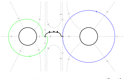
- [§4.3, proof of Theorem 4.16 (even n case)] The proof that f_L and f_R have different spin classes for even n is incomplete. The passage after Figure 24 states: 'Since μ bounds a disk in L, so γ cannot bound a disk in L because it is only a part of μ. Therefore, [C] = [γ] ≠ 0 ∈ H_1(L,Z).' This inference is not valid: the fact that the full curve μ is null-homologous gives no control over the homology class of a loop formed from a proper subarc of μ after endpoints are identified. A loop contained in the graph μ∪η can be null-homologous even if neither μ nor η contributes a nonzero class, and conversely a subarc of μ can produce a nonzero class only for reasons that are not supplied. Since for even n this is the only step distinguishing the two spin classes of framings, Theorem 4.16 is not fully proved as written. Example 4.18(ii) verifies only L(4,1) and does not close the gap.
- [§4.3, construction of the curve C] The topological construction of the Poincaré dual curve C is described too loosely. The text says that C_2, an arc in η, is 'shrunk to a point that identifies ξ_2 and ξ_2′' and that this is an isotopy, but an embedded arc with distinct endpoints cannot be shrunk to a point by an ambient isotopy of a 3-manifold; at best the described operation is a homotopy, and its effect on the homology class of the resulting loop is not justified. The paper should either replace this by a direct computation of [C] in H_1(L(n,k)) (for example, via the intersection form on the Heegaard torus or via the known classification of spin structures on lens spaces) or give a fully precise chain-level argument. This is load-bearing for the even-n case of the main theorem.
minor comments (4)
- [§4.3] The use of [23, Lem. 2.14] should be explained in more detail: the manuscript should state explicitly how the relative characteristic class c−c′ is represented by the closed curve C on which b_1 = −b_1′, and how the orientation and basepoint choices in Figures 23 and 24 determine a well-defined homology class.
- [§7, proof of Theorem 7.3] The proof of gauge invariance in Theorem 7.3 is a very long sequence of tensor manipulations with no intermediate named identities or checkpoints. I did not identify a specific error, but the exposition would be much more auditable if the cancellations were organized into lemmas or summarized in an appendix.
- [Throughout] There are numerous typos and small grammatical errors, including 'the the horizontal green line' in Section 4 and 'tothe' in the caption of Figure 11. A careful proofreading pass is needed.
- [§6, Theorem 6.2] The proof of gauge invariance of ν~_{n,k}(H) is concise but hard to follow at the step where Lemma 5.2(iii) is 'applied repeatedly'; please indicate explicitly which indices are being reduced at each application.
Circularity Check
No circularity: gauge invariance is derived from a direct trace identity, not from the result being proved.
full rationale
The paper's central claims are established by direct computation rather than by assuming what they prove. For the diagram framings f_R and f_L, the Kuperberg invariant is first expressed as Tr(S ∘ P^{(n,-k)}) (Theorem 4.9), and Theorem 4.10 then shows Tr(S ∘ P) = Tr(S_F ∘ P_F) for every 2-cocycle F, using Radford's trace formula and explicit cocycle identities that are proved in Section 5. The f_L case is reduced to f_R via the opposite Hopf algebra in Proposition 4.12, and the genus-2 result in Theorem 7.3 follows the same pattern. Since the paper's definition of gauge invariant (Definition 2.6) is exactly invariance under Drinfeld twists, this proves the claim from the stated input, not from the target result. Citations to prior work by one of the authors, such as [14] and [44], are used as external benchmarks or for standard elementary facts about 2-cocycles and indicators, and they are not load-bearing substitutes for the paper's own trace computations. The only questionable passage is the even-n spin-class argument at the end of Theorem 4.16, where the inference that a subarc of the null-homologous curve µ gives a nonzero loop γ is not justified; however, this is a correctness gap in a specific topological lemma, not a circular reduction, because the spin-class conclusion is not assumed in the premises and the independent numerical evidence in Example 4.18(ii) is presented as consistency rather than as an input to the proof. Overall, no construction in the paper reduces by definition or by self-citation to its own inputs.
Assumptions & free parameters
assumptions (4)
- domain assumption Two finite-dimensional Hopf algebras H and H' have equivalent tensor categories of representations if and only if H' is a Drinfeld twist of H by a 2-cocycle.
- standard math Radford's trace formula and the integral identities in Theorem 2.3 (i)-(vi) hold for arbitrary finite-dimensional Hopf algebras.
- domain assumption Kuperberg's construction gives a well-defined invariant of framed 3-manifolds that is independent of the framed Heegaard diagram, including invariance under base point isotopy and stabilization moves.
- standard math Obstruction theory classifies framings up to homotopy by H^1(M,Z/2) x H^3(M,Z) relative to a fixed framing, with the H^3 component called the Hopf degree.
Cite this review
Pith. "Pith review of Generalizations of Frobenius-Schur indicators from Kuperberg invariants." pith.science (2026). https://pith.science/paper/BOMMPEW2
@misc{pith2026250607409,
  author       = {Pith},
  title        = {Pith review of: Generalizations of Frobenius-Schur indicators from Kuperberg invariants},
  year         = {2026},
  howpublished = {\url{https://pith.science/paper/BOMMPEW2}},
  note         = {Machine review of arXiv:2506.07409}
}
abstract
We introduce an approach to produce gauge invariants of any finite-dimensional Hopf algebras from the Kuperberg invariants of framed 3-manifolds. These invariants are generalizations of Frobenius-Schur indicators of Hopf algebras. The computation of Kuperberg invariants is based on a presentation of the framed 3-manifold in terms of Heegaard diagram with combings satisfying certain admissibility conditions. We provide framed Heegaard diagrams for two infinite families of small genus 3-manifolds, which include all the lens spaces, and some homology spheres. In particular, the invariants of the lens spaces $L(n,1)$ coincide with the higher Frobenius-Schur indicators of Hopf algebras. We compute the Kuperberg invariants of all these framed 3-manifolds, and prove that they are invariants of the tensor category of representations of the underlying Hopf algebra, or simply gauge invariants.
Figures


Figures from the paper (21 more)



Reference graph
Works this paper leans on
-
[1]
E. Aljadeff, P. Etingof, S. Gelaki, and D. Nikshych. On twi sting of finite-dimensional Hopf algebras. J. Algebra, 256(2):484–501, 2002
work page 2002
-
[2]
L. Chang and Z. Wang. |ZKup| = |ZHenn|2 for lens spaces. Quantum Topol., 4(4):411–445, 2013
work page 2013
-
[3]
Q. Chen and T. Kerler. Integrality and gauge dependence o f Hennings TQFTs. J. Pure Appl. Algebra , 221(11):2689–2751, 2017
work page 2017
- [4]
-
[5]
P. Etingof and S. Gelaki. On finite-dimensional semisimp le and cosemisimple Hopf algebras in positive charac- teristic. Internat. Math. Res. Notices , (16):851–864, 1998
work page 1998
-
[6]
P. Etingof and S. Gelaki. On families of triangular Hopf a lgebras. Int. Math. Res. Not. , 2002(14):757–768, 2002
work page 2002
-
[7]
Etingof and V
P. Etingof and V. Ostrik. Finite tensor categories. Mosc. Math. J. , 4(3):627–654, 782–783, 2004
2004
-
[8]
R. Fenn and C. Rourke. On Kirby’s calculus of links. Topology, 18(1):1–15, 1979
work page 1979
Show all 47 references
-
[9]
Frobenius and I
G. Frobenius and I. Schur. ¨Uber die reellen darstellungen der endlichen gruppen. Sitzungsberichte der K¨ oniglich Preussischen Akademie der Wissenschaften , pages 186–208, 1906
1906
-
[10]
Fuchs, A
J. Fuchs, A. C. Ganchev, K. Szlach´ anyi, and P. Vecserny ´ es.S4 symmetry of 6 j symbols and Frobenius-Schur indicators in rigid monoidal C ∗ categories. J. Math. Phys. , 40(1):408–426, 1999
1999
-
[11]
Fuchs and C
J. Fuchs and C. Schweigert. Category theory for conform al boundary conditions. In Vertex operator algebras in mathematics and physics (Toronto, ON, 2000) , volume 39 of Fields Inst. Commun. , pages 25–70. Amer. Math. Soc., 2003
2000
-
[12]
P. M. Gilmer and J. M. Harris. On the kauffman bracket skei n module of the quaternionic manifold. J. Knot Theory Ramifications, 16(1):103–125, 2007
2007
-
[13]
Hennings
M. Hennings. Invariants of links and 3-manifolds obtai ned from Hopf algebras. J. London Math. Soc. (2) , 54(3):594–624, 1996
1996
-
[14]
Kashina, S
Y. Kashina, S. Montgomery, and S.-H. Ng. On the trace of t he antipode and higher indicators. Israel J. Math. , 188:57–89, 2012
2012
-
[15]
Kashina, Y
Y. Kashina, Y. Sommerh¨ auser, and Y. Zhu. On higher Frob enius-Schur indicators. Mem. Amer. Math. Soc. , 181(855):viii+65, 2006
2006
-
[16]
C. Kassel. Quantum groups, volume 155 of Graduate Texts in Mathematics . Springer-Verlag, New York, 1995
1995
-
[17]
L. H. Kauffman and D. E. Radford. Invariants of 3-manifol ds derived from finite-dimensional Hopf algebras. J. Knot Theory Ramifications , 4(1):131–162, 1995
1995
-
[18]
R. Kirby. A calculus for framed links in S3. Invent. Math. , 45(1):35–56, 1978
1978
-
[19]
Kuperberg
G. Kuperberg. Involutory Hopf algebras and 3-manifold invariants. Internat. J. Math. , 2(1):41–66, 1991
1991
-
[20]
Kuperberg
G. Kuperberg. Noninvolutory Hopf algebras and 3-manif old invariants. Duke Math. J. , 84(1):83–129, 1996
1996
-
[21]
R. G. Larson and D. E. Radford. Finite-dimensional cose misimple Hopf algebras in characteristic 0 are semisim- ple. J. Algebra, 117(2):267–289, 1988
1988
-
[22]
R. G. Larson and D. E. Radford. Semisimple cosemisimple Hopf algebras. Amer. J. Math. , 110(1):187–195, 1988
1988
-
[23]
C. Lescop. On homotopy invariants of combings of three- manifolds. Canad. J. Math. , 67(1):152–183, 2015. 57
2015
-
[24]
Linchenko and S
V. Linchenko and S. Montgomery. A Frobenius-Schur theo rem for Hopf algebras. Algebr. Represent. Theory , 3(4):347–355, 2000. Special issue dedicated to Klaus Rogge nkamp on the occasion of his 60th birthday
2000
-
[25]
Z. Liu, S. Ming, Y. Wang, and J. Wu. Alterfold toplogical quantum field theory. arXiv preprint arXiv:2312.06477 , 2023
2023 arXiv
-
[26]
S. Majid. Foundations of quantum group theory . Cambridge University Press, Cambridge, 1995
1995
-
[27]
Mason and S.-H
G. Mason and S.-H. Ng. Central invariants and Frobenius -Schur indicators for semisimple quasi-Hopf algebras. Adv. Math. , 190(1):161–195, 2005
2005
-
[28]
Matveev and M
S. Matveev and M. Polyak. A geometrical presentation of the surface mapping class group and surgery. Commun. Math. Phys. , 160(3):537–550, 1994
1994
-
[29]
J. Milnor. On the 3-dimensional Brieskorn manifolds M (p, q, r). In Knots, groups, and 3-manifolds (Papers dedicated to the memory of R. H. Fox) , Ann. of Math. Stud., No. 84, pages 175–225. Princeton Univ. Press, Princeton, NJ, 1975
1975
-
[30]
Montgomery
S. Montgomery. Hopf algebras and their actions on rings , volume 82 of CBMS Regional Conference Series in Mathematics. Published for the Conference Board of the Mathematical Sci ences, Washington, DC, 1993
1993
-
[31]
Montgomery
S. Montgomery. Representation theory of semisimple Ho pf algebras. In Algebra—representation theory (Con- stanta, 2000) , volume 28 of NATO Sci. Ser. II Math. Phys. Chem. , pages 189–218. Kluwer Acad. Publ., Dor- drecht, 2001
2000
-
[32]
Ng and P
S.-H. Ng and P. Schauenburg. Frobenius-Schur indicato rs and exponents of spherical categories. Adv. Math. , 211(1):34–71, 2007
2007
-
[33]
Ng and P
S.-H. Ng and P. Schauenburg. Central invariants and hig her indicators for semisimple quasi-Hopf algebras. Trans. Amer. Math. Soc. , 360(4):1839–1860, 2008
2008
-
[34]
W. D. Nichols and M. B. Zoeller. A Hopf algebra freeness t heorem. Amer. J. Math. , 111(2):381–385, 1989
1989
-
[35]
P. Orlik. Seifert manifolds . Lecture Notes in Mathematics, Vol. 291. Springer-Verlag, Berlin-New York, 1972
1972
-
[36]
D. E. Radford. The order of the antipode of a finite dimens ional Hopf algebra is finite. Amer. J. Math. , 98(2):333– 355, 1976
1976
-
[37]
D. E. Radford. The group of automorphisms of a semisimpl e Hopf algebra over a field of characteristic 0 is finite. Amer. J. Math. , 112(2):331–357, 1990
1990
-
[38]
D. E. Radford. The trace function and Hopf algebras. J. Algebra, 163(3):583–622, 1994
1994
-
[39]
Raymond and A
F. Raymond and A. T. Vasquez. 3-manifolds whose univers al coverings are Lie groups. Topology Appl., 12(2):161– 179, 1981
1981
-
[40]
Reidemeister
K. Reidemeister. Zur dreidimensionalen Topologie. Abh. Math. Sem. Univ. Hamburg , 9(1):189–194, 1933
1933
-
[41]
D. Rolfsen. Knots and links. Publish or Perish, Inc., Berkeley, Calif., 1976
1976
-
[42]
Saveliev
N. Saveliev. Lectures on the topology of 3-manifolds . De Gruyter Textbook. Walter de Gruyter & Co., Berlin, revised edition, 2012. An introduction to the Casson invari ant
2012
-
[43]
Schauenburg
P. Schauenburg. Hopf bi-Galois extensions. Comm. Algebra, 24(12):3797–3825, 1996
1996
-
[44]
K. Shimizu. On indicators of Hopf algebras. Israel J. Math. , 207(1):155–201, 2015
2015
-
[45]
J. Singer. Three-dimensional manifolds and their Heeg aard diagrams. Trans. Amer. Math. Soc. , 35(1):88–111, 1933
1933
-
[46]
M. E. Sweedler. Cohomology of algebras over Hopf algebr as. Trans. Amer. Math. Soc. , 133:205–239, 1968
1968
-
[47]
E. J. Taft. The order of the antipode of finite-dimension al Hopf algebra. Proc. Nat. Acad. Sci. U.S.A. , 68:2631– 2633, 1971. 58 Nankai University, School of Mathematical Sciences and LPM C, Tianjin, China Email address : changliang996@nankai.edu.cn Louisiana State University,...
1971
Reviewed August 7, 2026 · model on record in the stance chip above.
Discussion (0). Continue with ORCID to comment.