A Census of Variable Radio Sources at 3\,GHz
Pith reviewed 2026-05-22 00:13 UTC · model grok-4.3
The pith
About 3600 compact radio sources vary significantly over 2.5 years between VLASS epochs at 3 GHz.
A machine-rendered reading of the paper's core claim, the machinery that carries it, and where it could break.
Core claim
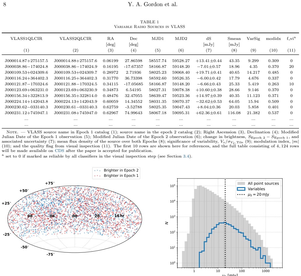
Approximately 3600 compact sources are found to significantly vary in brightness during the ~2.5 years between VLASS observations. For objects detected in both epochs whose mean flux density μ_S is brighter than 20 mJy, 5% show brightness variations >30%, rising to 9% at μ_S >300 mJy. Most variables have multiwavelength characteristics consistent with blazars and quasars, with blazars overrepresented and producing the largest absolute flux changes while galactic sources exhibit the largest fractional changes. More than 10,000 additional variables may exist among single-epoch detections.
What carries the argument
Flux density comparison between two VLASS epochs separated by ~2.5 years to identify significant variability among compact sources detected in both epochs.
Load-bearing premise
The measured flux differences between the two VLASS epochs reflect real astrophysical variability rather than residual calibration differences, imaging artifacts, or selection effects.
What would settle it
Re-observe a sample of the identified variable sources with an independent radio telescope to confirm whether the flux changes are repeatable and not due to calibration or artifacts.
Figures


read the original abstract
A wide range of phenomena, from explosive transients to active galactic nuclei, exhibit variability at radio wavelengths on timescales of a few years. Characterizing the rate and scale of variability in the radio sky can provide keen insights into dynamic processes in the Universe, such as accretion mechanics, jet propagation, and stellar evolution. We use data from the first two epochs of the Very Large Array Sky Survey (VLASS) to conduct a census of the variable radio sky. Approximately $3,600$ compact sources are found to significantly vary in brightness during the $\sim2.5\,$ years between observations. In this work we focus on sources that are detected in both VLASS epochs, but estimate there may be $>10,000$ additional variable radio sources in VLASS that are only detected in either the first or second epoch. For objects detected in both epochs whose mean flux density across the two epochs, $\mu_{S}$, is brighter than $20\,$mJy, $5\,$% show brightness variations $>30\,$%, rising to $9\,$% at $\mu_{S}>300\,$mJy. We analyze the redshift distributions, infrared colors, and $\gamma$-ray properties of the variable radio sources, finding that most have multiwavelength characteristics that are consistent with blazars and quasars. Blazars in particular are found to be overrepresented among the variable radio sources, and the largest absolute changes in flux density are produced by blazars. The largest fractional changes in brightness are exhibited by galactic sources. We discuss our results, including some of the more interesting and extreme examples of variable radio sources identified, as well as future research directions.
Editorial analysis
A structured set of objections, weighed in public.
Referee Report
Summary. The manuscript reports a census of variable radio sources at 3 GHz using the first two epochs of the VLASS survey. It identifies approximately 3,600 compact sources that significantly vary in brightness over the ~2.5 years between observations. For sources detected in both epochs with mean flux density μ_S > 20 mJy, 5% exhibit brightness variations exceeding 30%, increasing to 9% for μ_S > 300 mJy. The variable sources are analyzed for their multiwavelength properties, showing consistency with blazars and quasars, with blazars overrepresented and showing the largest absolute flux changes.
Significance. If the reported variability is astrophysical rather than due to systematics, this study offers a substantial statistical sample for understanding radio variability in AGN and other sources. The large number of variables and the multiwavelength cross-matching provide a foundation for future targeted studies of extreme variables. The direct use of survey data without additional modeling is a positive aspect.
major comments (2)
- [§3] §3 (Data and Methods): The precise definition of 'significantly vary' used to select the ~3,600 sources, including the exact significance threshold, handling of upper limits, and any post-selection cuts on the compact-source catalog, is not fully specified. This is load-bearing for interpreting the reported fractions and assessing selection biases.
- [§4.2] §4.2 (Variability Statistics): The headline result that 5% (9%) of sources with μ_S >20 mJy (>300 mJy) show >30% brightness variations assumes |S1−S2| reflects astrophysical changes. No control measurement of the flux-ratio distribution is reported for a large high-S/N compact-source sample selected to be non-variable by independent criteria, leaving open the possibility that residual epoch-to-epoch calibration offsets or imaging artifacts contribute to the high-variability tail.
minor comments (2)
- [Abstract] The estimate of >10,000 additional variables detected in only one epoch is stated without a quantitative justification or uncertainty estimate.
- Figure labels and captions could more explicitly indicate the variability thresholds used in the analysis.
Simulated Author's Rebuttal
We thank the referee for their careful and constructive review. We address each major comment below and have revised the manuscript to improve clarity on selection criteria and to include additional checks against systematics.
read point-by-point responses
-
Referee: [§3] §3 (Data and Methods): The precise definition of 'significantly vary' used to select the ~3,600 sources, including the exact significance threshold, handling of upper limits, and any post-selection cuts on the compact-source catalog, is not fully specified. This is load-bearing for interpreting the reported fractions and assessing selection biases.
Authors: We agree that the variability selection criteria should be stated more explicitly. In the revised manuscript we have expanded §3 with the precise definition: a source is included in the ~3600 sample if it is detected above 5σ in both epochs and satisfies |S1 − S2| / √(σ1² + σ2²) > 5, where the uncertainties include both statistical and a 3% systematic floor. Sources detected in only one epoch are treated as upper limits and are excluded from the main statistics (though we separately estimate >10,000 additional variables). Post-selection cuts on the compact catalog are now listed explicitly: peak-to-integrated flux ratio < 1.3 in both epochs, S/N > 7 on the mean flux, and removal of sources within 5 arcmin of bright extended emission. These additions allow full reproduction of the sample and direct assessment of selection biases. revision: yes
-
Referee: [§4.2] §4.2 (Variability Statistics): The headline result that 5% (9%) of sources with μ_S >20 mJy (>300 mJy) show >30% brightness variations assumes |S1−S2| reflects astrophysical changes. No control measurement of the flux-ratio distribution is reported for a large high-S/N compact-source sample selected to be non-variable by independent criteria, leaving open the possibility that residual epoch-to-epoch calibration offsets or imaging artifacts contribute to the high-variability tail.
Authors: We acknowledge the value of an independent control. While the significance threshold already folds in measurement uncertainties, we have added to the revised §4.2 a control sample of ~8000 high-S/N compact sources that lack Fermi-LAT γ-ray counterparts and exhibit quiescent WISE colors inconsistent with blazars. The flux-ratio distribution of this control sample is narrow (σ ≈ 0.12) with negligible tail beyond 30% variation, whereas the variable sample shows a clear excess. We also note that VLASS epoch-to-epoch calibration stability is documented at the ~2–3% level in the survey papers; residual systematics are therefore unlikely to dominate the reported high-variability tail. These additions directly address the concern. revision: yes
Circularity Check
Direct empirical census from survey data with no self-referential derivations
full rationale
The paper reports an observational census of variable sources by comparing flux densities between two independent VLASS epochs, counting sources that exceed a variability threshold. The headline fractions (5% and 9% of sources with μ_S >20 mJy or >300 mJy showing >30% changes) are direct empirical tallies from the catalog, not outputs of any fitted model, self-defined parameter, or self-citation chain that loops back to the same measurements. Multiwavelength characterizations draw on external catalogs. No load-bearing step in the provided text reduces a result to a definition or fit constructed from the variability data itself.
Axiom & Free-Parameter Ledger
free parameters (2)
- mean flux threshold
- variability significance cut
axioms (2)
- domain assumption Flux density differences between epochs are dominated by source variability rather than calibration or imaging differences
- domain assumption Compact sources detected in both epochs form an unbiased sample for variability statistics
Lean theorems connected to this paper
-
IndisputableMonolith/Foundation/RealityFromDistinction.leanreality_from_one_distinction unclear?
unclearRelation between the paper passage and the cited Recognition theorem.
We use data from the first two epochs of the Very Large Array Sky Survey (VLASS) to conduct a census of the variable radio sky. Approximately 3,600 compact sources are found to significantly vary...
-
IndisputableMonolith/Cost/FunctionalEquation.leanwashburn_uniqueness_aczel unclear?
unclearRelation between the paper passage and the cited Recognition theorem.
Vs = ΔS / σΔS ... and consider a source to be variable if it satisfies Vs > 4σVs,Tile ... |m| > 0.26
What do these tags mean?
- matches
- The paper's claim is directly supported by a theorem in the formal canon.
- supports
- The theorem supports part of the paper's argument, but the paper may add assumptions or extra steps.
- extends
- The paper goes beyond the formal theorem; the theorem is a base layer rather than the whole result.
- uses
- The paper appears to rely on the theorem as machinery.
- contradicts
- The paper's claim conflicts with a theorem or certificate in the canon.
- unclear
- Pith found a possible connection, but the passage is too broad, indirect, or ambiguous to say the theorem truly supports the claim.
Reference graph
Works this paper leans on
-
[1]
2020, ApJS, 247, 33, doi: 10.3847/1538-4365/ab6bcb
Abdollahi, S., Acero, F., Ackermann, M., et al. 2020, ApJS, 247, 33, doi: 10.3847/1538-4365/ab6bcb
-
[2]
2022, ApJS, 260, 53, doi: 10.3847/1538-4365/ac6751
Abdollahi, S., Acero, F., Baldini, L., et al. 2022, ApJS, 260, 53, doi: 10.3847/1538-4365/ac6751
-
[3]
2020, ApJS, 249, 3, doi: 10.3847/1538-4365/ab929e
Ahumada, R., Allende Prieto, C., Almeida, A., et al. 2020, ApJS, 249, 3, doi: 10.3847/1538-4365/ab929e
-
[4]
Aller, M. F., Aller, H. D., Hughes, P. A., & Latimer, G. E. 1999, ApJ, 512, 601, doi: 10.1086/306799
-
[5]
Anderson, M. M., Mooley, K. P., Hallinan, G., et al. 2020, ApJ, 903, 116, doi: 10.3847/1538-4357/abb94b
-
[6]
Andersson, A., Fender, R. P., Lintott, C. J., et al. 2022, MNRAS, 513, 3482, doi: 10.1093/mnras/stac1002
-
[7]
Assef, R. J., Stern, D., Kochanek, C. S., et al. 2013, ApJ, 772, 26, doi: 10.1088/0004-637X/772/1/26 Astropy Collaboration, Robitaille, T. P., Tollerud, E. J., et al. 2013, A&A, 558, A33, doi: 10.1051/0004-6361/201322068 Astropy Collaboration, Price-Whelan, A. M., Sip˝ ocz, B. M., et al. 2018, AJ, 156, 123, doi: 10.3847/1538-3881/aabc4f Astropy Collaborat...
work page internal anchor Pith review doi:10.1088/0004-637x/772/1/26 2013
-
[8]
Ball, L., Campbell-Wilson, D., Crawford, D. F., & Turtle, A. J. 1995, ApJ, 453, 864, doi: 10.1086/176446
-
[9]
Fermi Large Area Telescope Fourth Source Catalog Data Release 4 (4FGL-DR4)
Ballet, J., Bruel, P., Burnett, T. H., Lott, B., & The Fermi-LAT collaboration. 2023, arXiv e-prints, arXiv:2307.12546, doi: 10.48550/arXiv.2307.12546
work page internal anchor Pith review Pith/arXiv arXiv doi:10.48550/arxiv.2307.12546 2023
-
[10]
Banfield, J. K., Wong, O. I., Willett, K. W., et al. 2015, MNRAS, 453, 2326, doi: 10.1093/mnras/stv1688
-
[11]
Becker, R. H., White, R. L., & Helfand, D. J. 1995, ApJ, 450, 559, doi: 10.1086/176166
-
[12]
Bell, M. E., Murphy, T., Hancock, P. J., et al. 2019, MNRAS, 482, 2484, doi: 10.1093/mnras/sty2801
-
[13]
Bellm, E. C., Kulkarni, S. R., Graham, M. J., et al. 2019, PASP, 131, 018002, doi: 10.1088/1538-3873/aaecbe
-
[14]
Bhattacharya, D., & van den Heuvel, E. P. J. 1991, Phys. Rep., 203, 1, doi: 10.1016/0370-1573(91)90064-S
-
[15]
Blanton, M. R., Bershady, M. A., Abolfathi, B., et al. 2017, AJ, 154, 28, doi: 10.3847/1538-3881/aa7567
-
[16]
2012, in Astronomical Society of the Pacific Conference Series, Vol
Boch, T., Pineau, F., & Derriere, S. 2012, in Astronomical Society of the Pacific Conference Series, Vol. 461, Astronomical Data Analysis Software and Systems XXI, ed. P. Ballester, D. Egret, & N. P. F. Lorente, 291
work page 2012
-
[17]
2019, MNRAS, 482, 2, doi: 10.1093/mnras/sty2603
Bonaldi, A., Bonato, M., Galluzzi, V., et al. 2019, MNRAS, 482, 2, doi: 10.1093/mnras/sty2603
-
[18]
Bruzewski, S., Schinzel, F. K., Taylor, G. B., & Petrov, L. 2021, ApJ, 914, 42, doi: 10.3847/1538-4357/abf73b
-
[19]
2011, PASA, 28, 128, doi: 10.1071/AS10046
Cameron, E. 2011, PASA, 28, 128, doi: 10.1071/AS10046
-
[20]
Cendes, Y., Berger, E., Alexander, K. D., et al. 2024, ApJ, 971, 185, doi: 10.3847/1538-4357/ad5541
-
[21]
Condon, J. J. 1992, ARA&A, 30, 575, doi: 10.1146/annurev.aa.30.090192.003043
-
[22]
Condon, J. J., Cotton, W. D., Greisen, E. W., et al. 1998, AJ, 115, 1693, doi: 10.1086/300337
-
[23]
Condon, J. J., Matthews, A. M., & Broderick, J. J. 2019, ApJ, 872, 148, doi: 10.3847/1538-4357/ab0301
-
[24]
Cutri, R. M., Wright, E. L., Conrow, T., et al. 2014, VizieR Online Data Catalog: AllWISE Data Release (Cutri+ 2013), VizieR On-line Data Catalog: II/328. Originally published in: IPAC/Caltech (2013)
work page 2014
-
[25]
2022, ApJ, 931, L14, doi: 10.3847/2041-8213/ac6f08 de Menezes, R., Pe˜ na-Herazo, H
Darling, J. 2022, ApJ, 931, L14, doi: 10.3847/2041-8213/ac6f08 de Menezes, R., Pe˜ na-Herazo, H. A., Marchesini, E. J., et al. 2019, A&A, 630, A55, doi: 10.1051/0004-6361/201936195 de Vries, W. H., Becker, R. H., White, R. L., & Helfand, D. J. 2004, AJ, 127, 2565, doi: 10.1086/383550
-
[26]
Dey, A., Schlegel, D. J., Lang, D., et al. 2019, AJ, 157, 168, doi: 10.3847/1538-3881/ab089d Di Mauro, M., Manconi, S., Zechlin, H. S., et al. 2018, ApJ, 856, 106, doi: 10.3847/1538-4357/aab3e5
-
[27]
Z., Hallinan, G., Nakar, E., et al
Dong, D. Z., Hallinan, G., Nakar, E., et al. 2021, Science, 373, 1125, doi: 10.1126/science.abg6037
-
[28]
N., Pritchard, J., Murphy, T., et al
Driessen, L. N., Pritchard, J., Murphy, T., et al. 2024, PASA, 41, e084, doi: 10.1017/pasa.2024.72
-
[29]
Duchesne, S. W., Grundy, J. A., Heald, G. H., et al. 2024, PASA, 41, e003, doi: 10.1017/pasa.2023.60
-
[30]
Duncan, K. J. 2022, MNRAS, 512, 3662, doi: 10.1093/mnras/stac608
-
[31]
2021, ApJ, 906, 10, doi: 10.3847/1538-4357/abc5b1
Egron, E., Pellizzoni, A., Righini, S., et al. 2021, ApJ, 906, 10, doi: 10.3847/1538-4357/abc5b1
-
[32]
Feldman, P. A., Taylor, A. R., Gregory, P. C., et al. 1978, AJ, 83, 1471, doi: 10.1086/112346
-
[33]
Fender, R. P., Belloni, T. M., & Gallo, E. 2004, MNRAS, 355, 1105, doi: 10.1111/j.1365-2966.2004.08384.x
-
[34]
Fernandez, L. C., Secrest, N. J., Johnson, M. C., et al. 2022, ApJ, 927, 18, doi: 10.3847/1538-4357/ac4b5f
-
[35]
Fiedler, R. L., Waltman, E. B., Spencer, J. H., et al. 1987, ApJS, 65, 319, doi: 10.1086/191228
-
[36]
Fleming, T. A., Green, R. F., Jannuzi, B. T., et al. 1993, AJ, 106, 1729, doi: 10.1086/116760
-
[37]
M., Fuhrmann, L., & Perucho, M
Fromm, C. M., Fuhrmann, L., & Perucho, M. 2015, A&A, 580, A94, doi: 10.1051/0004-6361/201424815 Gaia Collaboration, Prusti, T., de Bruijne, J. H. J., et al. 2016, A&A, 595, A1, doi: 10.1051/0004-6361/201629272 Gaia Collaboration, Vallenari, A., Brown, A. G. A., et al. 2023, A&A, 674, A1, doi: 10.1051/0004-6361/202243940
-
[38]
2003, MNRAS, 344, 1000, doi: 10.1046/j.1365-8711.2003.06897.x
Gallo, E., Fender, R. P., & Pooley, G. G. 2003, MNRAS, 344, 60, doi: 10.1046/j.1365-8711.2003.06791.x
-
[39]
Gordon, Y. A., O’Dea, C. P., Baum, S. A., et al. 2023a, ApJ, 948, L9, doi: 10.3847/2041-8213/accf0a
-
[40]
Gordon, Y. A., Boyce, M. M., O’Dea, C. P., et al. 2020, RNAAS, 4, 175, doi: 10.3847/2515-5172/abbe23 —. 2021, ApJS, 255, 30, doi: 10.3847/1538-4365/ac05c0
-
[41]
A., Rudnick, L., Andernach, H., et al
Gordon, Y. A., Rudnick, L., Andernach, H., et al. 2023b, ApJS, 267, 37, doi: 10.3847/1538-4365/acda30
-
[42]
Hajela, A., Mooley, K. P., Intema, H. T., & Frail, D. A. 2019, MNRAS, 490, 4898, doi: 10.1093/mnras/stz2918
-
[43]
Refractive Interstellar Scintillation of Extra-galactic Radio Sources I: Expectations
Hurley-Walker, N. 2019, arXiv e-prints, arXiv:1907.08395, doi: 10.48550/arXiv.1907.08395
work page internal anchor Pith review Pith/arXiv arXiv doi:10.48550/arxiv.1907.08395 2019
-
[44]
Hancock, P. J., Drury, J. A., Bell, M. E., Murphy, T., & Gaensler, B. M. 2016, MNRAS, 461, 3314, doi: 10.1093/mnras/stw1486
-
[45]
Hancock, P. J., Gaensler, B. M., & Murphy, T. 2013, ApJ, 776, 106, doi: 10.1088/0004-637X/776/2/106
-
[46]
Hardcastle, M. J., Horton, M. A., Williams, W. L., et al. 2023, A&A, 678, A151, doi: 10.1051/0004-6361/202347333
-
[47]
Harris, C. R., Millman, K. J., van der Walt, S. J., et al. 2020, Nature, 585, 357, doi: 10.1038/s41586-020-2649-2
-
[48]
Hjellming, R. M., Rupen, M. P., Mioduszewski, A. J., & Narayan, R. 2000, The Astronomer’s Telegram, 54, 1
work page 2000
-
[49]
2019, New A Rev., 87, 101541, doi: 10.1016/j.newar.2020.101541
Hovatta, T., & Lindfors, E. 2019, New A Rev., 87, 101541, doi: 10.1016/j.newar.2020.101541
-
[50]
2008, A&A, 485, 51, doi: 10.1051/0004-6361:200809806
Hovatta, T., Nieppola, E., Tornikoski, M., et al. 2008, A&A, 485, 51, doi: 10.1051/0004-6361:200809806
-
[51]
2007, A&A, 469, 899, doi: 10.1051/0004-6361:20077529
Hovatta, T., Tornikoski, M., Lainela, M., et al. 2007, A&A, 469, 899, doi: 10.1051/0004-6361:20077529
-
[52]
2021, A&A, 650, A83, doi: 10.1051/0004-6361/202039481
Hovatta, T., Lindfors, E., Kiehlmann, S., et al. 2021, A&A, 650, A83, doi: 10.1051/0004-6361/202039481
-
[53]
Hufnagel, B. R., & Bregman, J. N. 1992, ApJ, 386, 473, doi: 10.1086/171033
-
[54]
Hunter, J. D. 2007, Computing in Science and Engineering, 9, 90, doi: 10.1109/MCSE.2007.55 Ivezi´ c,ˇZ., Kahn, S. M., Tyson, J. A., et al. 2019, ApJ, 873, 111, doi: 10.3847/1538-4357/ab042c
-
[55]
H., Cohen, M., Masci, F., et al
Jarrett, T. H., Cohen, M., Masci, F., et al. 2011, ApJ, 735, 112, doi: 10.1088/0004-637X/735/2/112
-
[56]
Joye, W. A., & Mandel, E. 2003, in Astronomical Society of the Pacific Conference Series, Vol. 295, Astronomical Data Analysis Software and Systems XII, ed. H. E. Payne, R. I. Jedrzejewski, & R. N. Hook, 489
work page 2003
-
[57]
Kadowaki, L. H. S., de Gouveia Dal Pino, E. M., & Singh, C. B. 2015, ApJ, 802, 113, doi: 10.1088/0004-637X/802/2/113
-
[58]
2019, MNRAS, 487, 3914, doi: 10.1093/mnras/stz1564
Kathirgamaraju, A., Giannios, D., & Beniamini, P. 2019, MNRAS, 487, 3914, doi: 10.1093/mnras/stz1564
-
[59]
Kimball, A. E. 2017, VLASS Project Memo 7: VLASS Tiling and Sky Coverage, https: //library.nrao.edu/public/memos/vla/vlass/VLASS 007.pdf
work page 2017
-
[60]
Koljonen, K. I. I., & Maccarone, T. J. 2017, MNRAS, 472, 2181, doi: 10.1093/mnras/stx2106
-
[61]
M., Lindfors, E., Hovatta, T., et al
Kouch, P. M., Lindfors, E., Hovatta, T., et al. 2024, A&A, 690, A111, doi: 10.1051/0004-6361/202347624
-
[62]
2023, A&A, 674, A198, doi: 10.1051/0004-6361/202245691
Kukreti, P., Morganti, R., Tadhunter, C., & Santoro, F. 2023, A&A, 674, A198, doi: 10.1051/0004-6361/202245691
-
[63]
Kun, E., Bartos, I., Tjus, J. B., et al. 2021, ApJ, 911, L18, doi: 10.3847/2041-8213/abf1ec
-
[64]
2020, ApJ, 897, 128, doi: 10.3847/1538-4357/ab9598
Kunert-Bajraszewska, M., Wo lowska, A., Mooley, K., Kharb, P., & Hallinan, G. 2020, ApJ, 897, 128, doi: 10.3847/1538-4357/ab9598
-
[65]
Lacy, M., Patil, P., & Nyland, K. 2022, VLASS Project Memo 17: Characterization of VLASS Single Epoch Continuum Validation Products, https: //library.nrao.edu/public/memos/vla/vlass/VLASS 017.pdf
work page 2022
-
[66]
Lacy, M., Meyers, S. T., Chandler, C., et al. 2019, VLASS Project Memo #13: Pilot and Epoch 1 Quick Look Data Release, https: //library.nrao.edu/public/memos/vla/vlass/VLASS 013.pdf
work page 2019
-
[67]
Jansky Very Large Array Sky Survey (VLASS)
Lacy, M., Baum, S. A., Chandler, C. J., et al. 2020, PASP, 132, 035001, doi: 10.1088/1538-3873/ab63eb
-
[68]
2018, ApJ, 866, L22, doi: 10.3847/2041-8213/aae5f3
Sironi, L. 2018, ApJ, 866, L22, doi: 10.3847/2041-8213/aae5f3
-
[69]
Lintott, C. J., Schawinski, K., Slosar, A., et al. 2008, MNRAS, 389, 1179, doi: 10.1111/j.1365-2966.2008.13689.x
-
[70]
Martinez, M. N., Gordon, Y. A., Bechtol, K., et al. 2025, ApJ, 979, 132, doi: 10.3847/1538-4357/ad9c37
-
[71]
2009, A&A, 495, 691, doi: 10.1051/0004-6361:200810161
Massaro, E., Giommi, P., Leto, C., et al. 2009, A&A, 495, 691, doi: 10.1051/0004-6361:200810161
-
[72]
2015, Ap&SS, 357, 75, doi: 10.1007/s10509-015-2254-2
Massaro, E., Maselli, A., Leto, C., et al. 2015, Ap&SS, 357, 75, doi: 10.1007/s10509-015-2254-2
-
[73]
2012, ApJ, 750, 138, doi: 10.1088/0004-637X/750/2/138
Massaro, F., D’Abrusco, R., Tosti, G., et al. 2012, ApJ, 750, 138, doi: 10.1088/0004-637X/750/2/138
-
[74]
Max-Moerbeck, W., Hovatta, T., Richards, J. L., et al. 2014, MNRAS, 445, 428, doi: 10.1093/mnras/stu1749
-
[75]
McConnell, D., Hale, C. L., Lenc, E., et al. 2020, PASA, 37, e048, doi: 10.1017/pasa.2020.41
-
[76]
Miller-Jones, J. C. A., Blundell, K. M., Rupen, M. P., et al. 2004, ApJ, 600, 368, doi: 10.1086/379706
-
[77]
Mingo, B., Watson, M. G., Rosen, S. R., et al. 2016, MNRAS, 462, 2631, doi: 10.1093/mnras/stw1826
-
[78]
Mohan, N., & Rafferty, D. 2015, PyBDSF: Python Blob Detection and Source Finder, Astrophysics Source Code Library, record ascl:1502.007
work page 2015
-
[79]
Mooley, K. P., Frail, D. A., Ofek, E. O., et al. 2013, ApJ, 768, 165, doi: 10.1088/0004-637X/768/2/165
-
[80]
P., Hallinan, G., Bourke, S., et al
Mooley, K. P., Hallinan, G., Bourke, S., et al. 2016, ApJ, 818, 105, doi: 10.3847/0004-637X/818/2/105 22 Y. A. Gordon et al
discussion (0)
Sign in with ORCID, Apple, or X to comment. Anyone can read and Pith papers without signing in.