REVIEW 3 major objections 4 minor 52 references
C, N, Na, and K hold the key to first-star mass recovery.
Reviewed by Pith at T0; open to challenge. T0 means a machine referee read the full paper against a public rubric. the ladder, T0–T4 →
T0 review · deepseek-v4-flash
2026-08-02 19:20 UTC pith:VAHSSJ6M
load-bearing objection Careful in-sample simulation study that yields a useful element ranking and planning metric, but the quantitative precision claims are only as good as the HW10 grid. the 3 major comments →
Quantifying Element Importance for Mass Recovery from Population III Supernova Yield Fits
The pith
A machine-rendered reading of the paper's core claim, the machinery that carries it, and where it could break.
Core claim
On the paper's own terms, the central result is a quantitative, grid-wide ranking of elemental importance for progenitor mass recovery. The most consistently 'very important' elements are C, N, Na, and K; O, Al, Co, and Ni consistently improve recovery when present. The paper further constructs a smooth mapping from its fit-quality metric to the expected fractional mass error, showing that element sets at or above the medium-coverage baseline typically recover mass within about 20% for 75% of mock stars, and the high-coverage baseline, which corresponds to elements actually measurable today, recovers mass almost perfectly. The practical claim is that stellar archaeology, with current high-re
What carries the argument
The quantitative engine is a mass-recovery score. For each model in the adopted core-collapse supernova yield grid, 100 noisy mock observations are generated and refit; a recovery counts as correct if the fitted mass lies within 10% of the true mass. Each grid frame is scored by a weighted count of correct and incorrect recoveries, and the score averages those frames over mixing prescriptions. Element importance is measured by how far the score moves when one element is added to or removed from a baseline set. This add/remove experiment, repeated for low-, medium-, and high-coverage baselines, yields the element ranking and the mapping between the score and expected mass precision.
Load-bearing premise
The mock observations are generated from the same yield grid that is later used as the fitting search space, so the measured recovery quality is an in-sample self-consistency test; if those theoretical yields do not represent real Population III supernovae, the quantitative precision mapping and the 'current elements suffice' conclusion do not transfer to observations.
What would settle it
Generate mock observations from a different core-collapse supernova yield grid with different physical assumptions, then refit them using the original grid. If mass recovery precision degrades significantly or the element importance ranking shifts substantially, the paper's central claim is an artifact of using the same grid for both mock generation and fitting.
If this is right
- Observational programs can prioritize measuring C, N, Na, and K; the paper shows that K, often neglected in metal-poor star abundance studies, is a high-value addition.
- The score-to-precision mapping gives a quantitative planning tool: choose a target mass precision and success rate, read the required score, and select element sets that achieve it.
- Both light and iron-peak elements are needed, and odd-Z elements are critical, so survey designs should not restrict to even-Z elements only.
- The current measurable element set is sufficient for practical IMF constraints, so waiting for future instruments is not necessary.
- Element rankings are robust to changes in the metric definition and correctness threshold, according to the paper.
Where Pith is reading between the lines
- Inference: The element ranking is calibrated entirely inside one yield grid; a natural extension is to test whether the same hierarchy survives when mock observations are drawn from an independent grid or a semi-analytic model. The sensitivity of C, N, and O may be robust, but the specific role of K could be grid-specific.
- Inference: The global ranking averages over mass and energy, and the paper itself notes subregion analyses could reveal mass-dependent importance. A pragmatic follow-up is per-mass-bin rankings to guide observations targeting the low-mass cutoff that matters for reionization.
- Inference: The framework treats all elements with equal noise; in reality, K and N are harder to measure. Coupling the importance ranking with realistic per-element uncertainties could change the recommended measurement priorities.
- Inference: If real extremely metal-poor stars are fit using this element guidance, the inferred IMF can be compared with predictions from first-star formation simulations; a mismatch would localize where yield models break down.
Editorial analysis
A structured set of objections, weighed in public.
Referee Report
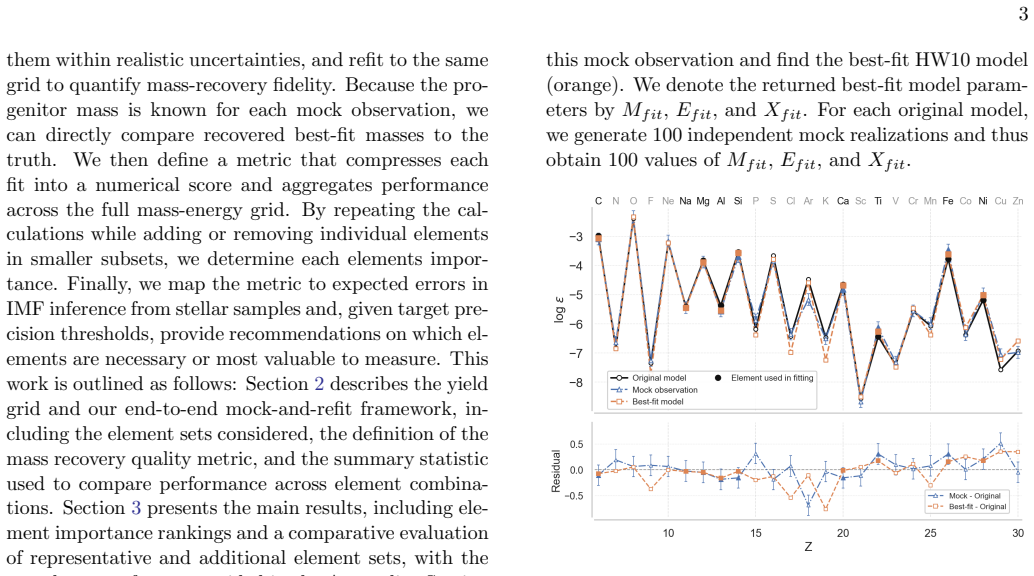
Summary. This paper presents a systematic, end-to-end mock-and-refit study to quantify which elements most control progenitor mass recovery when fitting Population III core-collapse supernova yields. Using the Heger & Woosley (2010, HW10) grid, the authors generate mock observations with Gaussian noise (σ=0.2 dex), fit them back to the same grid, and summarize recovery quality with a metric d̄. By adding/removing single elements from low-, medium-, and high-coverage baselines, they rank elements and identify C, N, Na, and K as consistently very important, with O, Al, Co, Ni also helpful. They then construct a d̄-to-δ mapping that relates fit quality to percentile fractional mass errors, and conclude that currently measurable elements from high-resolution spectroscopy can deliver practical Pop III IMF constraints, assuming the HW10 yields are representative. The analysis is thorough, with 100 mock realizations per model and tests of alternative metric choices.
Significance. If the results are robust, the paper provides the first quantitative element-importance ranking for Pop III mass recovery and a practical mapping from observed element sets to expected mass precision, which can guide observational campaigns and IMF inference. The controlled end-to-end pipeline, the explicit treatment of noise, and the robustness tests of the metric are strengths. However, the central quantitative claims are in-sample: mocks are drawn from and fit to the same HW10 grid, and all elements are assigned the same measurement uncertainty. These two assumptions directly affect both the element ranking and the precision mapping, so the practical conclusions require external validation or a more cautious framing. The authors acknowledge the single-grid limitation in Section 4, but the constant-noise assumption is not discussed as a limitation.
major comments (3)
- [Section 2.1 and 2.5] The mock observations are generated from HW10 and fit to the same HW10 grid, so the d̄-to-δ mapping and the near-perfect high-coverage recovery (Figures 5 and 6) are measures of self-consistency, not of performance under real yield-model errors. The paper's central claim that currently measurable elements can deliver practical IMF constraints depends on this mapping. Please either validate the ranking and δ percentiles with an independent yield grid (e.g., Nomoto et al. 2013 or Limongi & Chieffi 2018) or explicitly restrict all quantitative precision claims to 'within HW10' and add a quantitative discussion of how systematic errors in key elements would shift the mapping.
- [Section 2.1/2.2] The assumption that all elements have the same observational uncertainty σ=0.2 dex is unlikely to hold: elements such as K, Co, Ni, and N are typically harder to measure than Mg, Fe, or Ca, and many are only upper limits. Because the importance ranking is the paper's main output, the sensitivity of the ranking to element-dependent noise should be tested, e.g., by assigning larger σ to odd-Z/iron-peak elements and re-running the add/remove experiments. Without this, the recommendation to prioritize C, N, Na, K may not transfer to real spectra.
- [Section 2.4] The assignment of elements to 'very important' vs 'important' tiers is based on horizontal thresholds chosen by visual inspection of the Δd̄ values (Figure 4). Since the abstract's headline result is the identity of the most important elements, the thresholds should be justified quantitatively. Please report the numerical Δd̄ values (with scatter across the 14 mixing frames) and use a statistical criterion, e.g., a bootstrap confidence interval or a clustering algorithm, to define the tiers.
minor comments (4)
- [Section 3] The sentence 'the complete version of Figure 5 is provided in the Appendix' appears to refer to Figure 6 (element combinations), not Figure 5 (d̄-δ mapping). The appendix figure is labeled 'Full version of Figure 5' but shows element sets; update the cross-reference.
- [Section 2.5] There is a broken sentence: 'identify which element sets typically achieve that ¯d with Figure 5. Here we define...' This should be rephrased, likely as '...achieve that ¯d (Figure 6). Here we define...'.
- [Table 1] The red highlighting for Sc, Cr, Cu, Zn may not be distinguishable in black-and-white print; suggest using a symbol or a separate note.
- [Section 2.2] The exclusion of Sc, Cr, Cu, Zn is justified by HW10 modeling limitations, but the rationale could be expanded for readers unfamiliar with the starfit caveats.
Circularity Check
No circularity: the in-sample mock-and-refit framework is an explicit calibration, not an independent prediction, and the paper states its model-dependence as a limitation.
full rationale
The only potentially self-referential element is that mock observations are drawn from the Heger & Woosley (2010) grid and then fit to the same grid (Section 2.1). This is a controlled Monte Carlo calibration of the fitting procedure, not an independent validation of HW10 or an empirical prediction. The paper explicitly frames it that way: 'we address the question in a controlled setting: beginning with yield models rather than observations, we generate mock abundance vectors, perturb them within realistic uncertainties, and refit to the same grid to quantify mass-recovery fidelity.' The dbar-to-delta mapping is described as a calibration ('Our goal in this subsection is to calibrate the summary metric dbar to the expected uncertainty in progenitor mass recovery'), and the central conclusion is explicitly conditional: 'assuming the core-collapse supernova yield models provide a good representation of stellar evolution in the early universe.' Section 4 lists as a key limitation that 'all results are based on a single core-collapse supernova yield grid.' No fitted parameter is renamed as a prediction, no element importance is defined in terms of the conclusion, and no load-bearing uniqueness theorem, ansatz, or self-citation chain is used to force the result. The element rankings are a sensitivity analysis within a stated model assumption, so the derivation does not reduce to its own inputs by construction.
Axiom & Free-Parameter Ledger
free parameters (5)
- noise level sigma =
0.2 dex
- correctness threshold =
delta < 10%
- dbar category weights =
green 1, blue 0.5, yellow -0.5, red -1
- importance-tier thresholds =
visual cuts, different per baseline
- exponential percentile fits =
exponential curves fitted to 50/68/75/90th percentiles
axioms (4)
- domain assumption Heger & Woosley (2010) yield grid faithfully represents Population III core-collapse supernova nucleosynthesis.
- domain assumption Each extremely/ultra metal-poor star's heavy-element pattern comes from a single Population III star.
- domain assumption Independent Gaussian noise in logepsilon with sigma=0.2 adequately represents real abundance measurement uncertainties.
- domain assumption Minimizing chi-square over the HW10 grid is the appropriate way to recover progenitor mass.
read the original abstract
Massive Population III stars are currently not observed, but their initial mass function (IMF) can be inferred through stellar archaeology: fitting core-collapse supernova yield models to elemental abundances of low-mass, long-lived metal-poor stars. While prior work demonstrates that yield fitting can recover progenitor properties, it remains unclear which measured elements most control mass recovery quality and what level of IMF precision is achievable for a measured element set. We perform a systematic study of element importance for progenitor mass recovery. Using the Heger & Woosley (2010) yield grid, we generate mock observations, fit the initial mass, and evaluate the typical performance on the fractional mass recovery. Add/remove-one-element experiments and comparisons among different baseline element sets are used to rank elements by importance. We find that the most important elements for accurate mass recovery are C, N, Na, and K, with O, Al, Co, and Ni consistently improving performance when available. Overall, with currently measurable elements from high-resolution spectroscopy, stellar archaeology can deliver practical Population III IMF constraints assuming the core-collapse supernova yield models provide a good representation of stellar evolution in the early universe.
Figures


Reference graph
Works this paper leans on
-
[1]
Abel, T., Bryan, G. L., & Norman, M. L. 2002, Science, 295, 93, doi: 10.1126/science.1063991
-
[2]
2018, The Astrophysical Journal Supplement Series, 238, 36, doi: 10.3847/1538-4365/aadfe9 12
Abohalima, A., & Frebel, A. 2018, The Astrophysical Journal Supplement Series, 238, 36, doi: 10.3847/1538-4365/aadfe9 12
-
[3]
2001, Physics Reports, 349, 125, doi: https://doi.org/10.1016/S0370-1573(01)00019-9
Barkana, R., & Loeb, A. 2001, Physics Reports, 349, 125, doi: https://doi.org/10.1016/S0370-1573(01)00019-9
-
[4]
Beers, T. C., & Christlieb, N. 2005, Annual Review of Astronomy and Astrophysics, 43, 531, doi: https: //doi.org/10.1146/annurev.astro.42.053102.134057
arXiv 2005
-
[5]
2004, The Astrophysical Journal, 608, L45, doi: 10.1086/422172
Belczynski, K., Bulik, T., & Rudak, B. 2004, The Astrophysical Journal, 608, L45, doi: 10.1086/422172
doi:10.1086/422172 2004
-
[6]
Bessell, M. S., Collet, R., Keller, S. C., et al. 2015, The Astrophysical Journal Letters, 806, L16, doi: 10.1088/2041-8205/806/1/L16
-
[7]
2025, The most metal poor stars, https://arxiv.org/abs/2504.06335
Bonifacio, P., Caffau, E., Franois, P., & Spite, M. 2025, The most metal poor stars, https://arxiv.org/abs/2504.06335
Pith/arXiv arXiv 2025
-
[8]
2013, Reports on Progress in Physics, 76, 112901, doi: 10.1088/0034-4885/76/11/112901
Bromm, V. 2013, Reports on Progress in Physics, 76, 112901, doi: 10.1088/0034-4885/76/11/112901
-
[9]
Bromm, V., Coppi, P. S., & Larson, R. B. 1999, The Astrophysical Journal, 527, L5, doi: 10.1086/312385
doi:10.1086/312385 1999
-
[10]
Bromm, V., Coppi, P. S., & Larson, R. B. 2002b, The Astrophysical Journal, 564, 23, doi: 10.1086/323947
-
[11]
2004, A&A, 416, 1117, doi: 10.1051/0004-6361:20034074
Cayrel, R., Depagne, E., Spite, M., et al. 2004, A&A, 416, 1117, doi: 10.1051/0004-6361:20034074
-
[12]
R., Gilmore, G., Heger, A., & Chan, C
Fraser, M., Casey, A. R., Gilmore, G., Heger, A., & Chan, C. 2017, Monthly Notices of the Royal Astronomical Society, 468, 418, doi: 10.1093/mnras/stx480
-
[13]
Frebel, A., Chiti, A., Ji, A. P., Jacobson, H. R., & Placco, V. M. 2015, The Astrophysical Journal Letters, 810, L27, doi: 10.1088/2041-8205/810/2/L27
-
[14]
Frebel, A., & Norris, J. E. 2015, Annual Review of Astronomy and Astrophysics, 53, 631, doi: https: //doi.org/10.1146/annurev-astro-082214-122423
-
[15]
Greif, T. H., Glover, S. C. O., Bromm, V., & Klessen, R. S. 2010, The Astrophysical Journal, 716, 510, doi: 10.1088/0004-637X/716/1/510
-
[16]
J., Nordstrm, B., Bonifacio, P., et al
Hansen, C. J., Nordstrm, B., Bonifacio, P., et al. 2011, A&A, 527, A65, doi: 10.1051/0004-6361/201015076
-
[17]
N., Kobayashi, C., Tominaga, N., & Nomoto, K
Hartwig, T., Ishigaki, M. N., Kobayashi, C., Tominaga, N., & Nomoto, K. 2023, The Astrophysical Journal, 946, 20, doi: 10.3847/1538-4357/acbcc6
-
[18]
Hartwig, T., Lipatova, V., Glover, S. C. O., & Klessen, R. S. 2024, Monthly Notices of the Royal Astronomical Society, 535, 516, doi: 10.1093/mnras/stae2318
-
[19]
Heger, A., & Woosley, S. E. 2002, The Astrophysical Journal, 567, 532, doi: 10.1086/338487
doi:10.1086/338487 2002
-
[20]
Heger, A., & Woosley, S. E. 2010, The Astrophysical Journal, 724, 341, doi: 10.1088/0004-637X/724/1/341
-
[21]
2014, The Astrophysical Journal, 781, 60, doi: 10.1088/0004-637X/781/2/60
Hirano, S., Hosokawa, T., Yoshida, N., et al. 2014, The Astrophysical Journal, 781, 60, doi: 10.1088/0004-637X/781/2/60
-
[22]
Hosokawa, T., Omukai, K., Yoshida, N., & Yorke, H. W. 2011, Science, 334, 1250, doi: 10.1126/science.1207433
-
[23]
Hosokawa, T., Yoshida, N., Omukai, K., & Yorke, H. W. 2012, The Astrophysical Journal Letters, 760, L37, doi: 10.1088/2041-8205/760/2/L37
-
[24]
N., Tominaga, N., Kobayashi, C., & Nomoto, K
Ishigaki, M. N., Tominaga, N., Kobayashi, C., & Nomoto, K. 2014, The Astrophysical Journal Letters, 792, L32, doi: 10.1088/2041-8205/792/2/L32
-
[25]
N., Tominaga, N., Kobayashi, C., & Nomoto, K
Ishigaki, M. N., Tominaga, N., Kobayashi, C., & Nomoto, K. 2018, The Astrophysical Journal, 857, 46, doi: 10.3847/1538-4357/aab3de
-
[26]
Jiang, R., Li, H., Zhao, G., Xing, Q., & Xin, W. 2025, Abundance Pattern Fitting with Bayesian Inference: Constraining First Stars’ Properties and Their Explosion Mechanism with Extremely Metal-poor Stars, https://arxiv.org/abs/2510.05712
arXiv 2025
-
[27]
2024, The Astrophysical Journal, 976, 68, doi: 10.3847/1538-4357/ad808a
Jiang, R., Zhao, G., Li, H., & Xing, Q. 2024, The Astrophysical Journal, 976, 68, doi: 10.3847/1538-4357/ad808a
-
[28]
Karlsson, T., Bromm, V., & Bland-Hawthorn, J. 2013, Rev. Mod. Phys., 85, 809, doi: 10.1103/RevModPhys.85.809
-
[29]
2014, Monthly Notices of the Royal Astronomical Society, 442, 2963, doi: 10.1093/mnras/stu1022
Kinugawa, T., Inayoshi, K., Hotokezaka, K., Nakauchi, D., & Nakamura, T. 2014, Monthly Notices of the Royal Astronomical Society, 442, 2963, doi: 10.1093/mnras/stu1022
-
[30]
2015, Monthly Notices of the Royal Astronomical Society, 456, 1093, doi: 10.1093/mnras/stv2624
Kinugawa, T., Miyamoto, A., Kanda, N., & Nakamura, T. 2015, Monthly Notices of the Royal Astronomical Society, 456, 1093, doi: 10.1093/mnras/stv2624
-
[31]
2013, Stellar Structure and Evolution, doi: 10.1007/978-3-642-30304-3
Kippenhahn, R., Weigert, A., & Weiss, A. 2013, Stellar Structure and Evolution, doi: 10.1007/978-3-642-30304-3
-
[32]
Klessen, R. S., & Glover, S. C. O. 2023, The first stars: formation, properties, and impact, https://arxiv.org/abs/2303.12500
Pith/arXiv arXiv 2023
-
[33]
2012, A&A, 541, A120, doi: 10.1051/0004-6361/201118604
Kowalska, I., Bulik, T., & Belczynski, K. 2012, A&A, 541, A120, doi: 10.1051/0004-6361/201118604
-
[34]
2006, A&A, 459, 1001, doi: 10.1051/0004-6361:20065080
Kulczycki, K., Bulik, T., Belczyski, K., & Rudak, B. 2006, A&A, 459, 1001, doi: 10.1051/0004-6361:20065080
-
[35]
Magg, M., Nordlander, T., Glover, S. C. O., et al. 2020, Monthly Notices of the Royal Astronomical Society, 498, 3703, doi: 10.1093/mnras/staa2624
-
[36]
McKee, C. F., & Tan, J. C. 2008, The Astrophysical Journal, 681, 771, doi: 10.1086/587434
doi:10.1086/587434 2008
-
[37]
Nomoto, K., Kobayashi, C., & Tominaga, N. 2013, Annual Review of Astronomy and Astrophysics, 51, 457, doi: https://doi.org/10.1146/annurev-astro-082812- 140956 13
-
[38]
Nordlander, T., Bessell, M. S., DaCosta, G. S., et al. 2019, Monthly Notices of the Royal Astronomical Society: Letters, 488, L109, doi: 10.1093/mnrasl/slz109
-
[39]
Nordlander, T., Amarsi, A. M., Lind, K., et al. 2017, A&A, 597, A6, doi: 10.1051/0004-6361/201629202
-
[40]
OShea, B. W., & Norman, M. L. 2007, The Astrophysical Journal, 654, 66, doi: 10.1086/509250
doi:10.1086/509250 2007
-
[41]
Placco, V. M., Frebel, A., Lee, Y. S., et al. 2015, The Astrophysical Journal, 809, 136, doi: 10.1088/0004-637X/809/2/136
-
[42]
Placco, V. M., Frebel, A., Beers, T. C., et al. 2016, The Astrophysical Journal, 833, 21, doi: 10.3847/0004-637X/833/1/21
-
[43]
Placco, V. M., Roederer, I. U., Lee, Y. S., et al. 2021, The Astrophysical Journal Letters, 912, L32, doi: 10.3847/2041-8213/abf93d
-
[44]
Placco, V. M., Gupta, A. F., Almeida-Fernandes, F., et al. 2024, The Astrophysical Journal, 977, 12, doi: 10.3847/1538-4357/ad8646
-
[45]
M., Limberg, G., Chiti, A., et al
Placco, V. M., Limberg, G., Chiti, A., et al. 2025, The Astrophysical Journal, 991, 101, doi: 10.3847/1538-4357/adf846
-
[46]
2002, A&A, 382, 28, doi: 10.1051/0004-6361:20011619
Schaerer, D. 2002, A&A, 382, 28, doi: 10.1051/0004-6361:20011619
-
[47]
Sharda, P., Menon, S. H., Gerasimov, R., et al. 2025, Monthly Notices of the Royal Astronomical Society: Letters, 541, L1, doi: 10.1093/mnrasl/slaf043 Sk´ ulad´ ottir, ., Salvadori, S., Amarsi, A. M., et al. 2021, The Astrophysical Journal Letters, 915, L30, doi: 10.3847/2041-8213/ac0dc2
-
[48]
Stacy, A., Greif, T. H., & Bromm, V. 2012, Monthly Notices of the Royal Astronomical Society, 422, 290, doi: 10.1111/j.1365-2966.2012.20605.x
arXiv 2012
-
[49]
2014, The Astrophysical Journal, 792, 32, doi: 10.1088/0004-637X/792/1/32
Susa, H., Hasegawa, K., & Tominaga, N. 2014, The Astrophysical Journal, 792, 32, doi: 10.1088/0004-637X/792/1/32
-
[50]
2014, The Astrophysical Journal, 785, 98, doi: 10.1088/0004-637X/785/2/98
Tominaga, N., Iwamoto, N., & Nomoto, K. 2014, The Astrophysical Journal, 785, 98, doi: 10.1088/0004-637X/785/2/98
-
[51]
Tumlinson, J., Venkatesan, A., & Shull, J. M. 2004, The Astrophysical Journal, 612, 602, doi: 10.1086/422571
-
[52]
2008, Science, 321, 669, doi: 10.1126/science.1160259
Yoshida, N., Omukai, K., & Hernquist, L. 2008, Science, 321, 669, doi: 10.1126/science.1160259
discussion (0)
Sign in with ORCID, Apple, or X to comment. Anyone can read and Pith papers without signing in.