Recognition: 2 theorem links
· Lean TheoremRFOX (Rotated-Field Oscillatory eXchange) quantum algorithm: Towards Parameter-Free Quantum Optimizers
Pith reviewed 2026-05-13 20:18 UTC · model grok-4.3
The pith
The RFOX algorithm maintains an essentially flat spectral gap independent of interpolation parameter and disorder strength.
A machine-rendered reading of the paper's core claim, the machinery that carries it, and where it could break.
Core claim
RFOX combines an almost constant non-stoquastic XX catalyst with a weak harmonic ZX counter-diabatic term; the Floquet-Magnus expansion at high frequency produces an effective Hamiltonian whose first-order term keeps the full XX driver while the leading correction consists of local single-qubit Y fields and poly-local 3-body topological interactions, ensuring the instantaneous spectral gap remains essentially flat independent of the interpolation parameter and disorder strength, modulated only by δ.
What carries the argument
The high-frequency Floquet-Magnus effective Hamiltonian derived from the constant XX plus harmonic ZX driver, which generates gap-preserving corrections of local Y fields and 3-body terms.
If this is right
- RFOX attains near-optimal and sometimes exact ground states using up to an order of magnitude fewer Trotter slices than X, XX or X+sXX schedules.
- Runtime scales constantly as T proportional to the inverse square of the minimum gap.
- Performance advantage over conventional drivers grows with increasing disorder strength.
- Hardware runs on IBM processors with 12-20 qubits reproduce the same performance ranking.
Where Pith is reading between the lines
- Analytically derived counter-diabatic terms may stabilize gaps in other non-stoquastic drivers for larger combinatorial problems.
- The fixed-gap construction could reduce the need for instance-specific schedule tuning across different optimization classes.
- Similar Floquet-derived corrections might apply to adiabatic algorithms beyond the random-field Ising model.
Load-bearing premise
The Floquet-Magnus expansion at high drive frequency accurately captures the effective Hamiltonian such that the derived corrections preserve gap flatness for the full range of disorder strengths and system sizes.
What would settle it
Exact diagonalization or simulation showing significant gap narrowing or collapse for system sizes larger than 12 qubits at high disorder would falsify the essential flatness claim.
Figures


read the original abstract
We introduce RFOX (Rotated-Field Oscillatory eXchange), a parameter-free quantum algorithm for combinatorial optimization. RFOX combines an almost constant non-stoquastic $XX$ catalyst with a weak harmonic $ZX$ counter-diabatic term. Using the Floquet-Magnus expansion, we derive a closed-form effective Hamiltonian whose first-order term retains the full $XX$ driver, while the leading correction consists of a local single-qubit $Y$ field and poly-local 3-body topological interactions driven by the graph connectivity at high drive frequency. This structure ensures that the instantaneous spectral gap remains essentially flat, independent of both the interpolation parameter and the disorder strength, modulated only by a $\delta$ parameter. This behavior stands in stark contrast to the unpredictable gap reductions, or even collapses, exhibited by the $X$ (stoquastic), $XX$, and $X+sXX$ (non-stoquastic) driver schedules. Extensive noiseless simulations on random-field Ising model (RFIM) instances with 7, 9, and 12 qubits, across three magnetic-field ranges, validate these spectral predictions: RFOX attains near-optimal, and in some cases exact, ground states using up to an order of magnitude fewer Trotter slices. Its performance advantage grows with increasing disorder, as conventional methods slow down near vanishing gaps, whereas RFOX maintains a constant runtime scaling of $T \propto \Delta_{\min}^{-2}$. Hardware experiments on IBM Quantum processors (Eagle r3 and Heron r1, with 12, 15, and 20 physical qubits) reproduce similar performance rankings. These results suggest that fixed-gap, non-stoquastic drivers augmented with analytically derived counter-diabatic terms offer a promising, scalable, and tuning-free route toward quantum optimizers for combinatorial optimization problems.
Editorial analysis
A structured set of objections, weighed in public.
Referee Report
Summary. The manuscript introduces the RFOX quantum algorithm for combinatorial optimization, combining a nearly constant non-stoquastic XX catalyst with a weak harmonic ZX counter-diabatic term. Via the Floquet-Magnus expansion, it derives a closed-form effective Hamiltonian whose leading term retains the full XX driver while corrections consist of local Y fields and 3-body interactions. This structure is claimed to produce an essentially flat instantaneous spectral gap independent of the interpolation parameter s and disorder strength (modulated only by δ), in contrast to X, XX, and X+sXX drivers. The claims are supported by noiseless simulations on RFIM instances with 7, 9, and 12 qubits across three field ranges, demonstrating near-optimal ground states with up to an order of magnitude fewer Trotter slices and constant runtime scaling T ∝ Δ_min^{-2}, plus hardware runs on IBM Eagle and Heron processors with 12-20 qubits that reproduce the performance ranking.
Significance. If the flat-gap property holds beyond the simulated regimes, the result would be significant for quantum optimization. It provides a parameter-free, analytically derived non-stoquastic driver that avoids the gap closures typical of standard schedules, with constant runtime scaling and hardware validation. The combination of Floquet-Magnus derivation with explicit counter-diabatic terms and reproducible simulation/hardware comparisons is a clear strength that could inform scalable quantum solvers for combinatorial problems.
major comments (3)
- [Abstract / Floquet-Magnus derivation] Abstract and derivation section: The central claim that the instantaneous gap remains essentially flat (independent of s and disorder strength) is derived from the leading-order Floquet-Magnus effective Hamiltonian. No explicit bounds or estimates are given on the remainder of the Magnus series, which is required to confirm that O(1/ω) and higher corrections do not induce gap dependence for strong disorder where local field scales increase.
- [Simulation results] Simulation results: The noiseless simulations on 7-12 qubit RFIM instances support the performance advantage and constant scaling, but report no error bars on success probabilities or runtime metrics and provide no finite-size scaling analysis, leaving open whether gap flatness and the T ∝ Δ_min^{-2} scaling survive at larger N or stronger disorder.
- [Hardware experiments] Hardware experiments: The IBM device runs (12-20 qubits) reproduce the ranking, but the manuscript supplies no quantitative description of error mitigation, readout calibration, or how the observed advantage scales with noise strength, which is load-bearing for claims of practical relevance.
minor comments (1)
- [Abstract] The phrase 'poly-local 3-body topological interactions driven by the graph connectivity' would benefit from an explicit operator example or diagram to clarify the structure of the correction terms.
Simulated Author's Rebuttal
We thank the referee for their constructive and positive assessment of our manuscript on the RFOX algorithm. We address each major comment point by point below, providing clarifications and indicating where revisions will be incorporated to strengthen the presentation.
read point-by-point responses
-
Referee: [Abstract / Floquet-Magnus derivation] Abstract and derivation section: The central claim that the instantaneous gap remains essentially flat (independent of s and disorder strength) is derived from the leading-order Floquet-Magnus effective Hamiltonian. No explicit bounds or estimates are given on the remainder of the Magnus series, which is required to confirm that O(1/ω) and higher corrections do not induce gap dependence for strong disorder where local field scales increase.
Authors: We agree that explicit estimates on the Magnus remainder would reinforce the flat-gap claim. In the revised manuscript we will add a dedicated paragraph in the derivation section that bounds the leading O(1/ω) correction for the chosen drive frequency ω ≫ local-field scale. We will show analytically that these corrections remain local and s-independent to first order, and we will include numerical checks on small instances confirming that gap flatness is preserved up to moderate disorder strengths. This addition directly addresses the concern without altering the core result. revision: yes
-
Referee: [Simulation results] Simulation results: The noiseless simulations on 7-12 qubit RFIM instances support the performance advantage and constant scaling, but report no error bars on success probabilities or runtime metrics and provide no finite-size scaling analysis, leaving open whether gap flatness and the T ∝ Δ_min^{-2} scaling survive at larger N or stronger disorder.
Authors: We will augment the simulation figures with error bars obtained from 50 independent random instances per size and field range. A new paragraph will be added discussing finite-size trends: while exhaustive scaling at N>12 is computationally prohibitive at present, the effective-Hamiltonian derivation is size-independent in the leading Magnus term, and the observed constant scaling T ∝ Δ_min^{-2} is consistent across the simulated range. We therefore view the current data as supportive but will explicitly note the limitation and the need for future larger-N studies. revision: partial
-
Referee: [Hardware experiments] Hardware experiments: The IBM device runs (12-20 qubits) reproduce the ranking, but the manuscript supplies no quantitative description of error mitigation, readout calibration, or how the observed advantage scales with noise strength, which is load-bearing for claims of practical relevance.
Authors: We will expand the hardware section with a quantitative description of the error-mitigation pipeline, including standard Qiskit readout-error calibration matrices applied to all devices and the number of shots used. We will also report the measured advantage (success probability ratio) as a function of device-reported two-qubit gate error rates across Eagle and Heron processors, thereby demonstrating that the performance ordering persists under realistic noise levels. revision: yes
Circularity Check
No significant circularity in the derivation chain
full rationale
The paper derives the effective Hamiltonian via the standard Floquet-Magnus expansion applied to the RFOX driver (XX catalyst plus weak ZX term). The flat-gap claim is presented as a direct consequence of the analytically obtained structure of this effective Hamiltonian (retained full XX term plus derived local-Y and 3-body corrections), not as a self-definition or post-hoc fit. The modulation parameter δ emerges from the expansion rather than being tuned to enforce flatness. No load-bearing self-citations, uniqueness theorems, or ansatzes imported from prior author work are invoked to force the result. Small-scale simulations serve as external validation of the derived spectral behavior, not as input that defines it. The chain is therefore self-contained.
Axiom & Free-Parameter Ledger
free parameters (1)
- δ
axioms (1)
- domain assumption Floquet-Magnus expansion yields an accurate closed-form effective Hamiltonian at high drive frequency
Lean theorems connected to this paper
-
IndisputableMonolith/Cost/FunctionalEquation.leanwashburn_uniqueness_aczel unclear?
unclearRelation between the paper passage and the cited Recognition theorem.
Using the Floquet-Magnus expansion, we derive a closed-form effective Hamiltonian whose first-order term retains the full XX driver, while the leading correction consists of a local single-qubit Y field and poly-local 3-body topological interactions... This structure ensures that the instantaneous spectral gap remains essentially flat, independent of both the interpolation parameter and the disorder strength, modulated only by a delta parameter.
-
IndisputableMonolith/Foundation/RealityFromDistinction.leanreality_from_one_distinction unclear?
unclearRelation between the paper passage and the cited Recognition theorem.
RFOX maintains a constant runtime scaling of T proportional to Delta_min^{-2}.
What do these tags mean?
- matches
- The paper's claim is directly supported by a theorem in the formal canon.
- supports
- The theorem supports part of the paper's argument, but the paper may add assumptions or extra steps.
- extends
- The paper goes beyond the formal theorem; the theorem is a base layer rather than the whole result.
- uses
- The paper appears to rely on the theorem as machinery.
- contradicts
- The paper's claim conflicts with a theorem or certificate in the canon.
- unclear
- Pith found a possible connection, but the passage is too broad, indirect, or ambiguous to say the theorem truly supports the claim.
Reference graph
Works this paper leans on
-
[1]
String-overlap fidelity To quantify performance, we compute the string-overlap fidelity between the most frequently observed bitstring (the winner) and the theoretical ground-state bitstring (gs): Foverlap = 1 − dH(winner, gs) n , (37) where n = 12 and the Hamming distance given by dH(g, w) = nX i=1 (1 − δgi,wi) = nX i=1 |gi − wi|, (38) with gi, wi ∈ { 0,...
-
[2]
Distribution overlap via Jensen–Shannon distance Continuing our analysis, we compute the Jensen–Shannon distance between the hardware output distribution p and the simulated distribution q: DJS(p ∥ q) = 1 2 DKL(p ∥ m) + DKL(q ∥ m) , m = 1 2(p + q) , (39) where the Kullback-Leibler divergence is DKL(k ∥ m) =P x∈X k(x) log k(x) m(x), with k equal to p or q....
-
[3]
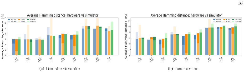
Figure 11 displays the resulting distributions
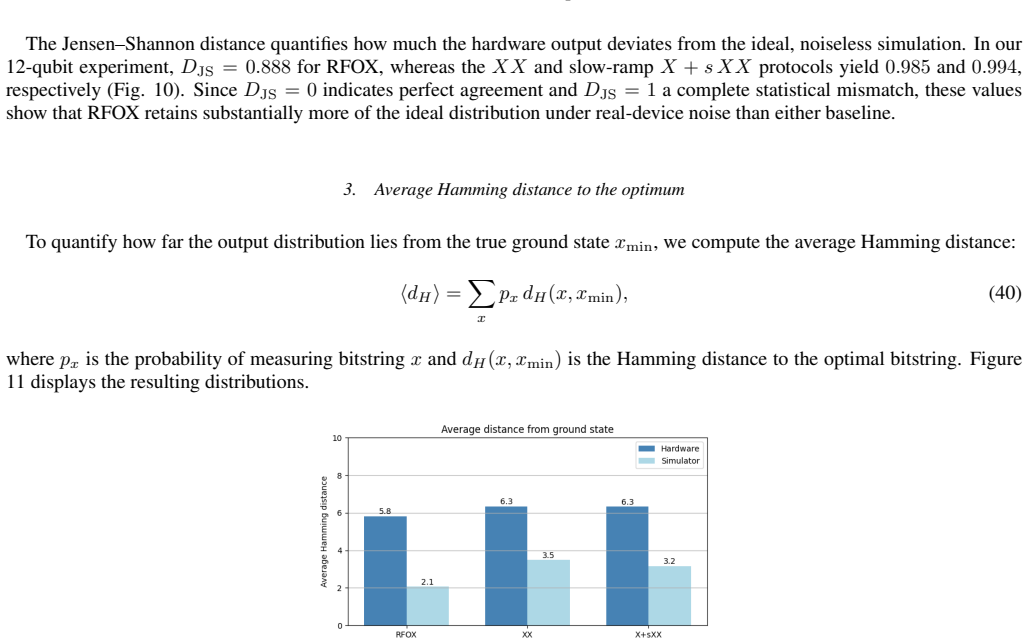
Average Hamming distance to the optimum To quantify how far the output distribution lies from the true ground state xmin, we compute the average Hamming distance: ⟨dH ⟩ = X x px dH(x, xmin), (40) where px is the probability of measuring bitstring x and dH(x, xmin) is the Hamming distance to the optimal bitstring. Figure 11 displays the resulting distribut...
-
[4]
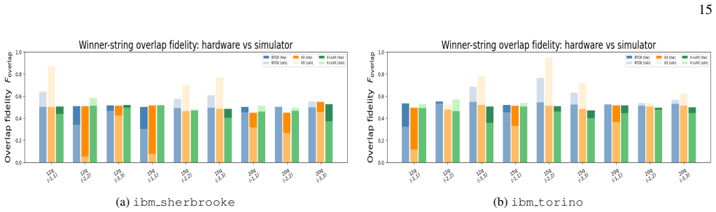
RFIM experiments on ibm sherbrooke and ibm torino For the final results, we generated random RFIM instances on the IBM Quantum backends ibm sherbrooke and ibm torino, using N ∈ {12, 15, 20} physical qubits and field ranges[−1, 1], [−2, 2], and [−3, 3]. We fixed the CD amplitude at δ = 0.001 (matching the simulation) and employed p = 50 time-slices for bot...
-
[5]
A variational eigenvalue solver on a photonic quantum processor,
A. Peruzzo, J. McClean, P. Shadbolt, M.-H. Yung, X.-Q. Zhou, P. J. Love, A. Aspuru-Guzik, and J. L. O’brien, “A variational eigenvalue solver on a photonic quantum processor,”Nature communications, vol. 5, no. 1, p. 4213, 2014
work page 2014
-
[6]
Vqe method: a short survey and recent developments,
D. A. Fedorov, B. Peng, N. Govind, and Y . Alexeev, “Vqe method: a short survey and recent developments,” Materials Theory, vol. 6, no. 1, p. 2, 2022
work page 2022
-
[7]
Layer vqe: A variational approach for combinatorial optimization on noisy quantum computers,
X. Liu, A. Angone, R. Shaydulin, I. Safro, Y . Alexeev, and L. Cincio, “Layer vqe: A variational approach for combinatorial optimization on noisy quantum computers,”IEEE Transactions on Quantum Engineering, vol. 3, pp. 1–20, 2022
work page 2022
-
[8]
A Quantum Approximate Optimization Algorithm
E. Farhi, J. Goldstone, and S. Gutmann, “A quantum approximate optimization algorithm,” arXiv preprint arXiv:1411.4028, 2014
work page internal anchor Pith review Pith/arXiv arXiv 2014
-
[9]
A review on quantum approximate optimization algorithm and its variants,
K. Blekos, D. Brand, A. Ceschini, C.-H. Chou, R.-H. Li, K. Pandya, and A. Summer, “A review on quantum approximate optimization algorithm and its variants,”Physics Reports, vol. 1068, pp. 1–66, 2024
work page 2024
-
[10]
L. Zhou, S.-T. Wang, S. Choi, H. Pichler, and M. D. Lukin, “Quantum approximate optimization algorithm: Performance, mechanism, and implementation on near-term devices,”Physical Review X, vol. 10, no. 2, p. 021067, 2020
work page 2020
-
[11]
Qaoa-in-qaoa: solving large-scale maxcut problems on small quantum machines,
Z. Zhou, Y . Du, X. Tian, and D. Tao, “Qaoa-in-qaoa: solving large-scale maxcut problems on small quantum machines,”Physical Review Applied, vol. 19, no. 2, p. 024027, 2023
work page 2023
-
[12]
Performance of the quantum approximate optimization algorithm on the maximum cut problem,
G. E. Crooks, “Performance of the quantum approximate optimization algorithm on the maximum cut problem,” arXiv preprint arXiv:1811.08419, 2018
-
[13]
Recursive qaoa outperforms the original qaoa for the max-cut problem on complete graphs,
E. Bae and S. Lee, “Recursive qaoa outperforms the original qaoa for the max-cut problem on complete graphs,” Quantum Information Processing, vol. 23, no. 3, p. 78, 2024
work page 2024
-
[14]
Quantum computing in the NISQ era and beyond,
J. Preskill, “Quantum computing in the NISQ era and beyond,” Quantum, vol. 2, p. 79, 2018
work page 2018
-
[15]
A variational eigenvalue solver on a photonic quantum processor,
A. Peruzzo, J. R. McClean, P. Shadbolt, M.-H. Yung, X.-Q. Zhou, P. J. Love, A. Aspuru-Guzik, and J. L. O’Brien, “A variational eigenvalue solver on a photonic quantum processor,”Nature Communications, vol. 5, p. 4213, 2014
work page 2014
-
[16]
Variational quantum algorithms,
M. Cerezo, A. Arrasmith, R. Babbush, S. C. Benjamin, S. Endo, K. Fujii, C. Hempel, S. Im, Z. Jiang, J. R. McClean, K. Mitarai, X. Yuan, L. Cincio, and P. J. Coles, “Variational quantum algorithms,”Nature Reviews Physics, vol. 3, pp. 625–644, 2021
work page 2021
-
[17]
M. Motta, C. Sun, A. T. K. Tan, and other authors, “Determining eigenstates and thermal states on a quantum computer using quantum imaginary time evolution,”Nature Physics, vol. 16, pp. 205–210, 2020. 18
work page 2020
-
[18]
A fast quantum mechanical algorithm for database search,
L. K. Grover, “A fast quantum mechanical algorithm for database search,” in Proceedings of the twenty-eighth annual ACM symposium on Theory of computing, 1996, pp. 212–219
work page 1996
-
[19]
Quantum computing for pattern classification,
M. Schuld, I. Sinayskiy, and F. Petruccione, “Quantum computing for pattern classification,” in PRICAI 2014: Trends in Artificial Intelligence: 13th Pacific Rim International Conference on Artificial Intelligence, Gold Coast, QLD, Australia, December 1-5, 2014. Proceedings 13. Springer, 2014, pp. 208–220
work page 2014
-
[20]
Optimal training of variational quantum algorithms without barren plateaus,
T. Haug and M. Kim, “Optimal training of variational quantum algorithms without barren plateaus,” arXiv preprint arXiv:2104.14543, 2021
-
[21]
Escaping from the barren plateau via gaussian initializations in deep variational quantum circuits,
K. Zhang, L. Liu, M.-H. Hsieh, and D. Tao, “Escaping from the barren plateau via gaussian initializations in deep variational quantum circuits,”Advances in Neural Information Processing Systems, vol. 35, pp. 18 612–18 627, 2022
work page 2022
-
[22]
Barren plateaus in quantum neural network training landscapes,
J. R. McClean, S. Boixo, V . N. Smelyanskiy, R. Babbush, and H. Neven, “Barren plateaus in quantum neural network training landscapes,” Nature Communications, vol. 9, p. 4812, 2018
work page 2018
-
[23]
Noise-induced barren plateaus in variational quantum algorithms,
X. Wang, M. Cerezo, P. J. Coles, and S. Lloyd, “Noise-induced barren plateaus in variational quantum algorithms,” Nature Communications, vol. 12, p. 6961, 2021
work page 2021
-
[24]
Quantum annealing of the random-field Ising model by transverse ferromagnetic interactions,
S. Suzuki, H. Nishimori, and M. Suzuki, “Quantum annealing of the random-field Ising model by transverse ferromagnetic interactions,” Physical Review E, vol. 75, p. 051112, 2007
work page 2007
-
[25]
Computational characteristics of random field ising model on quantum devices,
Y . Zhouet al., “Computational characteristics of random field ising model on quantum devices,”arXiv preprint arXiv:2205.13782, 2022
-
[26]
Optimal parameter initialization for qaoa via spectral analysis,
H. Yang et al., “Optimal parameter initialization for qaoa via spectral analysis,”arXiv preprint arXiv:2408.00557, 2024
-
[27]
Improving nonstoquastic quantum annealing with spin-reversal transformations,
E. M. Lykiardopoulou, A. Zucca, S. A. Scivier, and M. H. Amin, “Improving nonstoquastic quantum annealing with spin-reversal transformations,”Physical Review A, vol. 104, no. 1, p. 012619, 2021
work page 2021
-
[28]
Role of nonstoquastic catalysts in quantum adiabatic optimization,
T. Albash, “Role of nonstoquastic catalysts in quantum adiabatic optimization,” Physical Review A, vol. 99, no. 4, p. 042334, 2019
work page 2019
-
[29]
V . Choi, “Essentiality of the non-stoquastic hamiltonians and driver graph design in quantum optimization annealing,” arXiv preprint arXiv:2105.02110, 2021
-
[30]
An introduction to the ising model,
B. A. Cipra, “An introduction to the ising model,” The American Mathematical Monthly, vol. 94, no. 10, pp. 937–959, 1987
work page 1987
-
[31]
The ising model, computer simulation, and universal physics,
R. I. Hughes, “The ising model, computer simulation, and universal physics,” Ideas In Context, vol. 52, pp. 97–145, 1999
work page 1999
-
[32]
D. Ceperley and B. Alder, “Quantum monte carlo,” Science, vol. 231, no. 4738, pp. 555–560, 1986
work page 1986
-
[33]
Quantum monte carlo and related approaches,
B. M. Austin, D. Y . Zubarev, and W. A. Lester Jr, “Quantum monte carlo and related approaches,”Chemical reviews, vol. 112, no. 1, pp. 263–288, 2012
work page 2012
-
[34]
J. Gubernatis, N. Kawashima, and P. Werner, Quantum Monte Carlo Methods. Cambridge University Press, 2016
work page 2016
-
[35]
The Complexity of Stoquastic Local Hamiltonian Problems
S. Bravyi, D. P. Divincenzo, R. I. Oliveira, and B. M. Terhal, “The complexity of stoquastic local hamiltonian problems,” arXiv preprint quant-ph/0606140, 2006
work page internal anchor Pith review Pith/arXiv arXiv 2006
-
[36]
Monte carlo simulation of stoquastic hamiltonians,
S. Bravyi, “Monte carlo simulation of stoquastic hamiltonians,” arXiv preprint arXiv:1402.2295, 2014
-
[37]
Two-local qubit hamiltonians: when are they stoquastic?
J. Klassen and B. M. Terhal, “Two-local qubit hamiltonians: when are they stoquastic?” Quantum, vol. 3, p. 139, 2019
work page 2019
-
[38]
Nonstoquastic hamiltonians and quantum annealing of an ising spin glass,
L. Hormozi, E. W. Brown, G. Carleo, and M. Troyer, “Nonstoquastic hamiltonians and quantum annealing of an ising spin glass,”Physical review B, vol. 95, no. 18, p. 184416, 2017
work page 2017
-
[39]
On the computational complexity of curing the sign problem,
M. Marvian, D. A. Lidar, and I. Hen, “On the computational complexity of curing the sign problem,” arXiv preprint arXiv:1802.03408, 2018
-
[40]
Hardness and ease of curing the sign problem for two-local qubit hamiltonians,
J. Klassen, M. Marvian, S. Piddock, M. Ioannou, I. Hen, and B. M. Terhal, “Hardness and ease of curing the sign problem for two-local qubit hamiltonians,”SIAM Journal on Computing, vol. 49, no. 6, pp. 1332–1362, 2020
work page 2020
-
[41]
Termwise versus globally stoquastic local hamiltonians: questions of complexity and sign-curing,
M. Ioannou, S. Piddock, M. Marvian, J. Klassen, and B. M. Terhal, “Termwise versus globally stoquastic local hamiltonians: questions of complexity and sign-curing,”arXiv preprint arXiv:2007.11964, 2020
-
[42]
Non-stoquastic hamiltonians in quantum annealing via geometric phases,
W. Vinci and D. A. Lidar, “Non-stoquastic hamiltonians in quantum annealing via geometric phases,” npj Quantum Information, vol. 3, no. 1, p. 38, 2017
work page 2017
-
[43]
Exponential enhancement of the efficiency of quantum annealing by non-stoquastic hamiltonians,
H. Nishimori and K. Takada, “Exponential enhancement of the efficiency of quantum annealing by non-stoquastic hamiltonians,” Frontiers in ICT, vol. 4, p. 2, 2017
work page 2017
-
[44]
Nonstoquastic hamiltonians and quantum annealing of an ising spin glass,
L. Hormozi, E. W. Brown, G. Carleo, and M. Troyer, “Nonstoquastic hamiltonians and quantum annealing of an ising spin glass,” Phys. Rev. B, vol. 95, p. 184416, May 2017. [Online]. Available: https://link.aps.org/doi/10.1103/PhysRevB.95.184416
-
[45]
Shortcuts to adiabaticity for fast qubit readout in circuit quantum electrodynamics,
F. C ´ardenas-L´opez and X. Chen, “Shortcuts to adiabaticity for fast qubit readout in circuit quantum electrodynamics,” Physical Review Applied, vol. 18, no. 3, p. 034010, 2022
work page 2022
-
[46]
Floquet-engineering counterdiabatic protocols in quantum many-body systems,
P. W. Claeys, M. Pandey, D. Sels, and A. Polkovnikov, “Floquet-engineering counterdiabatic protocols in quantum many-body systems,” Physical review letters, vol. 123, no. 9, p. 090602, 2019
work page 2019
-
[47]
Photonic counterdiabatic quantum optimization algorithm,
P. Chandarana, K. Paul, M. Garcia-de Andoin, Y . Ban, M. Sanz, and X. Chen, “Photonic counterdiabatic quantum optimization algorithm,”Communications Physics, vol. 7, no. 1, p. 315, 2024
work page 2024
-
[48]
Minimizing irreversible losses in quantum systems by local counterdiabatic driving,
D. Sels and A. Polkovnikov, “Minimizing irreversible losses in quantum systems by local counterdiabatic driving,” Proceedings of the National Academy of Sciences, vol. 114, no. 20, pp. E3909–E3916, 2017
work page 2017
-
[49]
M. Bukov, L. D’Alessio, and A. Polkovnikov, “Universal high-frequency behavior of periodically driven systems: from dynamical stabilization to floquet engineering,”Advances in Physics, vol. 64, no. 2, pp. 139–226, 2015
work page 2015
-
[50]
Effects of xx catalysts on quantum annealing spectra with perturbative crossings,
N. Feinstein, L. Fry-Bouriaux, S. Bose, and P. Warburton, “Effects of xx catalysts on quantum annealing spectra with perturbative crossings,”Physical Review A, vol. 110, no. 4, p. 042609, 2024
work page 2024
-
[51]
The magnus expansion and some of its applications,
S. Blanes, F. Casas, J.-A. Oteo, and J. Ros, “The magnus expansion and some of its applications,” Physics reports, vol. 470, no. 5-6, pp. 151–238, 2009
work page 2009
-
[52]
T. Kuwahara, T. Mori, and K. Saito, “Floquet–magnus theory and generic transient dynamics in periodically driven many-body quantum systems,”Annals of Physics, vol. 367, pp. 96–124, 2016
work page 2016
-
[53]
Colloquium: Exactly solvable richardson-gaudin models for many-body quantum systems,
J. Dukelsky, S. Pittel, and G. Sierra, “Colloquium: Exactly solvable richardson-gaudin models for many-body quantum systems,”Reviews of modern physics, vol. 76, no. 3, pp. 643–662, 2004. 19
work page 2004
-
[54]
Geometric methods for nonlinear many-body quantum systems,
M. Lewin, “Geometric methods for nonlinear many-body quantum systems,” Journal of Functional Analysis, vol. 260, no. 12, pp. 3535– 3595, 2011
work page 2011
-
[55]
Relaxation times of dissipative many-body quantum systems,
M. ˇZnidariˇc, “Relaxation times of dissipative many-body quantum systems,”Physical Review E, vol. 92, no. 4, p. 042143, 2015
work page 2015
-
[56]
Quantum trajectories and open many-body quantum systems,
A. J. Daley, “Quantum trajectories and open many-body quantum systems,” Advances in Physics, vol. 63, no. 2, pp. 77–149, 2014
work page 2014
-
[57]
S. A. Weidinger and M. Knap, “Floquet prethermalization and regimes of heating in a periodically driven, interacting quantum system,” Scientific reports, vol. 7, no. 1, p. 45382, 2017
work page 2017
-
[58]
Floquet prethermalization in a bose-hubbard system,
A. Rubio-Abadal, M. Ippoliti, S. Hollerith, D. Wei, J. Rui, S. Sondhi, V . Khemani, C. Gross, and I. Bloch, “Floquet prethermalization in a bose-hubbard system,”Physical Review X, vol. 10, no. 2, p. 021044, 2020
work page 2020
-
[59]
Floquet prethermalization in dipolar spin chains,
P. Peng, C. Yin, X. Huang, C. Ramanathan, and P. Cappellaro, “Floquet prethermalization in dipolar spin chains,”Nature Physics, vol. 17, no. 4, pp. 444–447, 2021
work page 2021
-
[60]
Counterdiabatic driving for periodically driven systems,
P. M. Schindler and M. Bukov, “Counterdiabatic driving for periodically driven systems,” Physical Review Letters, vol. 133, no. 12, p. 123402, 2024. Appendix A: Magnetic field phase mapping We start from the all-zero state |ψ0⟩ =Nn i=1 |0⟩ and create a uniform superposition over all computational basis states by applying the Walsh-Hadamard transform to ea...
work page 2024
-
[61]
Phase encoding interference After encoding the local fields with phase gates, we apply a second layer of Hadamard gates H ⊗n. This step converts the encoded phases into amplitude variations, creating interference patterns that highlight the field contributions in the measurement basis. Concretely, if the system is initially in the state: |ψ2⟩ = 1√ 2n 2n−1...
discussion (0)
Sign in with ORCID, Apple, or X to comment. Anyone can read and Pith papers without signing in.