arxiv: 2604.02889 · v1 · submitted 2026-04-03 · 📊 stat.ML · cs.AI· cs.LG

Recognition: no theorem link

Rethinking Forward Processes for Score-Based Data Assimilation in High Dimensions

Eunbi Yoon , Donghan Kim , Dae Wook Kim

Authors on Pith no claims yet

Pith reviewed 2026-05-13 18:16 UTC · model grok-4.3

classification 📊 stat.ML cs.AIcs.LG

keywords score-based generative modelsdata assimilationBayesian filteringmeasurement-aware forward processlikelihood scorehigh-dimensional filteringposterior score

0 comments

The pith

A measurement-aware forward process built from the measurement equation yields exact likelihood scores for score-based data assimilation.

A machine-rendered reading of the paper's core claim, the machinery that carries it, and where it could break.

The paper proposes a measurement-aware score-based filter that constructs the forward diffusion process directly from the measurement equation rather than specifying it independently. This change renders the likelihood score analytically tractable, so that for linear measurements the exact likelihood score can be derived and added to a learned prior score to form the posterior score. A sympathetic reader would care because existing score-based filters rely on heuristic approximations of the likelihood score that accumulate error over sequential updates in high dimensions. The resulting method is tested on high-dimensional datasets and reported to improve accuracy and stability relative to prior score-based approaches.

Core claim

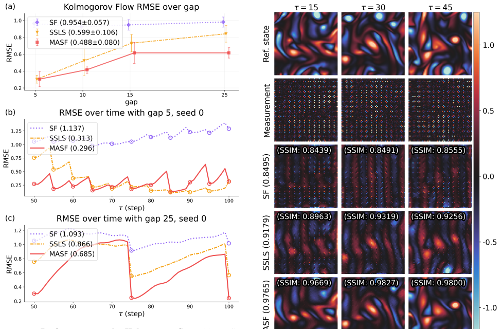
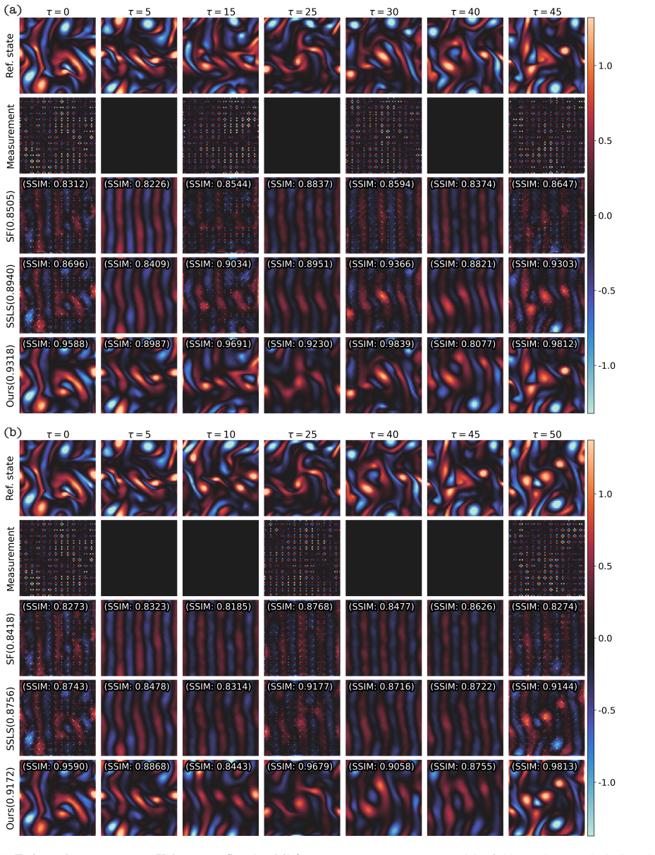
We propose a measurement-aware score-based filter (MASF) that defines a measurement-aware forward process directly from the measurement equation. This construction makes the likelihood score analytically tractable: for linear measurements, we derive the exact likelihood score and combine it with a learned prior score to obtain the posterior score.

What carries the argument

The measurement-aware forward process constructed directly from the measurement equation, which renders the likelihood score exact rather than approximate.

If this is right

The measurement-update step no longer relies on heuristic approximations of the likelihood score.
Posterior scores are formed by direct addition of an exact likelihood score and a learned prior score.
Error accumulation across sequential assimilation steps is reduced in high-dimensional settings.
Numerical experiments on high-dimensional datasets show gains in accuracy and stability over existing score-based filters.

Where Pith is reading between the lines

These are editorial extensions of the paper, not claims the author makes directly.

The construction may extend to mildly nonlinear measurements by retaining the same forward-process logic with local linearizations.
Long-horizon assimilation chains could see compounding benefits from the absence of per-step heuristic error.
The same measurement-aware principle might be tested in other generative-model-based filtering frameworks outside score-based diffusion.

Load-bearing premise

Building the forward process directly from the measurement equation preserves the diffusion properties required for stable score-based sampling and does not create new instabilities or extra approximation errors in high dimensions.

What would settle it

Run the proposed MASF and a standard score-based filter side-by-side on a high-dimensional linear measurement assimilation task and check whether the new method exhibits lower error accumulation or greater instability over long sequences.

Figures

Figures reproduced from arXiv: 2604.02889 by Dae Wook Kim, Donghan Kim, Eunbi Yoon.

**Figure 1.** Figure 1: Schematic comparison of likelihood score. (a) Existing approaches specify the forward process independently of the measurement equation, which makes the likelihood intractable. (b) Our approach aligns the forward process with the measurement equation, so the likelihood score becomes tractable. the measurement equation. Such filtering problems arise broadly in domains where time-evolving dynamics must be i… view at source ↗

**Figure 2.** Figure 2: Pipeline of the proposed method, MASF. The forward process is constructed by interpolating between the identity and the measurement operator, so that the state is progressively degraded toward the measurement. The reverse-time process samples state trajectories from the posterior. et al. [2021], Dhariwal and Nichol [2021]. These models learn the score function, the gradient of the log-density, and enable s… view at source ↗

**Figure 1.** Figure 1: In the linear measurement case, we construct the for [PITH_FULL_IMAGE:figures/full_fig_p002_1.png] view at source ↗

**Figure 3.** Figure 3: State trajectories for the Lorenz–63 system with measurement gap 100. Each panel shows the reference trajectory and the assimilated trajectory produced by one of the considered methods: (a) EnKF, (b) SF, (c) SSLS, and (d) MASF. The title of each subplot reports the trajectory RMSE for a representative run (seed 1), followed by the mean ± standard deviation of RMSE computed over five random seeds. Overall, … view at source ↗

**Figure 4.** Figure 4: Performance on the Lorenz–96 system across state dimension, chaoticity, and measurement sparsity. Panels (a)–(b) vary the state dimension, (c)–(d) vary the forcing parameter, and (e)–(f) vary the measurement gap, with the remaining parameters fixed as indicated in each panel title. Across all three sweeps, MASF achieves consistently lower RMSE and shows robust performance under variations in dimension, for… view at source ↗

**Figure 5.** Figure 5: Performance on the Kolmogorov flow. (a) RMSE as a function of the measurement gap. Points show the mean over 5 random seeds and error bars indicate ± standard deviation across seeds. (b,c) RMSE over time for representative runs at gap= 5 (b) and gap= 25 (c) with seed 0. Open circles denote measurement-update steps; numbers in parentheses report the timeaveraged RMSE for each method on the shown trajectory… view at source ↗

**Figure 7.** Figure 7: Additional qualitative results for different random seeds. Lorenz–63 state trajectories with measurement gap 100 for (a) EnKF, (b) SF, (c) SSLS, and (d) MASF. Each row corresponds to a different random seed (0, 2, 3, 4), showing the reference trajectory and the assimilated trajectory; subplot titles report the trajectory RMSE for each run. 20 [PITH_FULL_IMAGE:figures/full_fig_p020_7.png] view at source ↗

**Figure 8.** Figure 8: Estimated system state on Kolmogorov flow (seed 0) for two measurement gaps. Vorticity fields are shown at the indicated time indices τ . (a) gap= 5 and (b) gap= 10. Top to bottom: reference state, sparse measurement, and reconstructions by SF, SSLS, and MASF. Numbers in each reconstruction panel report the per-frame SSIM with respect to the reference at the same τ . 21 [PITH_FULL_IMAGE:figures/full_fig_p… view at source ↗

**Figure 9.** Figure 9: Estimated system state on Kolmogorov flow (seed 0) for two measurement gaps. Vorticity fields are shown at the indicated time indices τ . (a) gap= 15 and (b) gap= 25. Top to bottom: reference state, sparse measurement, and reconstructions by SF, SSLS, and MASF. Numbers in each reconstruction panel report the per-frame SSIM with respect to the reference at the same τ . 22 [PITH_FULL_IMAGE:figures/full_fig_… view at source ↗

read the original abstract

Data assimilation is the process of estimating the time-evolving state of a dynamical system by integrating model predictions and noisy observations. It is commonly formulated as Bayesian filtering, but classical filters often struggle with accuracy or computational feasibility in high dimensions. Recently, score-based generative models have emerged as a scalable approach for high-dimensional data assimilation, enabling accurate modeling and sampling of complex distributions. However, existing score-based filters often specify the forward process independently of the data assimilation. As a result, the measurement-update step depends on heuristic approximations of the likelihood score, which can accumulate errors and degrade performance over time. Here, we propose a measurement-aware score-based filter (MASF) that defines a measurement-aware forward process directly from the measurement equation. This construction makes the likelihood score analytically tractable: for linear measurements, we derive the exact likelihood score and combine it with a learned prior score to obtain the posterior score. Numerical experiments covering a range of settings, including high-dimensional datasets, demonstrate improved accuracy and stability over existing score-based filters.

Editorial analysis

A structured set of objections, weighed in public.

Desk editor's note, referee report, simulated authors' rebuttal, and a circularity audit. Tearing a paper down is the easy half of reading it; the pith above is the substance, this is the friction.

Desk Editor's Note private letter to a colleague

Tying the forward process to the measurement equation gives an exact likelihood score for linear cases, but whether this keeps the diffusion Markovian and stable in high dimensions is the part that still needs checking.

read the letter

The main new piece is defining the forward process directly from the measurement equation so the likelihood score becomes exact for linear observations instead of relying on heuristics. They then add this to a learned prior score to get the posterior. This targets a real limitation in earlier score-based filters where the forward process was chosen independently and error built up across steps. The abstract reports experiments on high-dimensional data that show better accuracy and stability, which is the right kind of test for this kind of work. If the numbers hold, it could be useful for people doing sequential estimation in complex dynamical systems. The soft spot is the diffusion structure itself. Adding measurement dependence to the forward SDE risks introducing extra drift or diffusion terms that could violate the conditions for a unique strong solution or clean time reversal. The stress-test note flags this, and without the full derivation it is not clear how they ensure the Fokker-Planck relation stays standard or that high-dimensional variance stays controlled. The abstract claims an exact derivation for linear measurements, but the details are not visible here, so the claim cannot be verified yet. No sign of circularity or obvious fitting problems. This is for researchers working on score-based generative models for data assimilation or high-dimensional filtering. A reader who already knows the score-based filter literature would get the most out of it. The idea is focused enough and the experiments are relevant enough that it deserves a serious referee to check the SDE construction and the quantitative results. I would send it to peer review rather than desk reject.

Referee Report

3 major / 2 minor

Summary. The manuscript proposes a measurement-aware score-based filter (MASF) for data assimilation that constructs the forward process directly from the linear measurement equation y = Hx + ε. This yields an exact, analytically tractable likelihood score that is added to a learned prior score to form the posterior score, with the claim that the approach improves accuracy and stability over existing score-based filters in high dimensions.

Significance. If the measurement-aware forward process preserves the Markov diffusion structure and the standard existence/uniqueness conditions for the reverse SDE, the method would reduce reliance on heuristic likelihood approximations and could deliver more reliable posterior sampling in high-dimensional assimilation tasks.

major comments (3)

[§3] The construction of the measurement-aware forward process (described in the abstract and §3) must explicitly verify that the resulting drift and diffusion coefficients satisfy the Lipschitz and linear-growth conditions required for a unique strong solution to the SDE; without this, the exact likelihood term does not automatically cancel potential non-Markovian artifacts or variance explosion in high dimensions.
[§4.1] The derivation of the exact likelihood score ∇ log p(y|x_t) for linear measurements (claimed in the abstract) is not reproduced in sufficient detail to confirm it follows directly from the measurement equation without additional approximations; the full steps, including the explicit form of the forward SDE and assumptions on H and ε, are needed to support the central claim.
[Experiments] High-dimensional numerical experiments must include diagnostics (e.g., trajectory variance, checks on marginal Fokker-Planck consistency, or Markov property preservation) to demonstrate that the new forward process does not introduce instabilities absent in standard score-based filters.

minor comments (2)

[Abstract] The abstract refers to 'a range of settings' without enumeration; listing the specific datasets or dimensions would improve clarity.
[Notation] Notation for the time-dependent coefficients in the forward process should be defined once and used consistently to avoid ambiguity when combining prior and likelihood scores.

Simulated Author's Rebuttal

3 responses · 0 unresolved

We thank the referee for the constructive comments on our manuscript. We address each major point below and have revised the manuscript to incorporate the requested clarifications, proofs, and diagnostics.

read point-by-point responses

Referee: [§3] The construction of the measurement-aware forward process (described in the abstract and §3) must explicitly verify that the resulting drift and diffusion coefficients satisfy the Lipschitz and linear-growth conditions required for a unique strong solution to the SDE; without this, the exact likelihood term does not automatically cancel potential non-Markovian artifacts or variance explosion in high dimensions.

Authors: We agree that explicit verification of the Lipschitz and linear-growth conditions is required for rigor. In the revised §3 we have added a dedicated subsection proving that, under the standing assumptions of a bounded linear operator H and Gaussian measurement noise ε with finite second moments, both the drift and diffusion coefficients of the measurement-aware forward process satisfy the global Lipschitz and linear-growth conditions. This guarantees a unique strong solution to the SDE and confirms that the exact likelihood score does not introduce non-Markovian artifacts or uncontrolled variance growth. revision: yes
Referee: [§4.1] The derivation of the exact likelihood score ∇ log p(y|x_t) for linear measurements (claimed in the abstract) is not reproduced in sufficient detail to confirm it follows directly from the measurement equation without additional approximations; the full steps, including the explicit form of the forward SDE and assumptions on H and ε, are needed to support the central claim.

Authors: We have expanded §4.1 with the complete derivation. Starting from the linear measurement model y = Hx + ε with ε ∼ N(0,R), the measurement-aware forward SDE is defined as dx_t = [f(x_t) + g(t)^2 H^T R^{-1}(y − H μ_t)] dt + g(t) dW_t, where μ_t is the conditional mean under the forward process. We then compute the conditional density p(y|x_t) explicitly, yielding the exact score ∇_x log p(y|x_t) = −H^T R^{-1}(H μ_t − y) with no further approximations. All assumptions (H linear and bounded, R positive definite and known) are now stated at the beginning of the section. revision: yes
Referee: [Experiments] High-dimensional numerical experiments must include diagnostics (e.g., trajectory variance, checks on marginal Fokker-Planck consistency, or Markov property preservation) to demonstrate that the new forward process does not introduce instabilities absent in standard score-based filters.

Authors: We agree that such diagnostics strengthen the empirical validation. The revised experiments section now includes (i) plots of trajectory variance versus time for all high-dimensional test cases, (ii) numerical residuals measuring consistency with the marginal Fokker–Planck equation, and (iii) empirical checks of the Markov property via conditional independence tests on sampled trajectories. These diagnostics show that the measurement-aware forward process introduces no additional instabilities relative to standard score-based filters. revision: yes

Circularity Check

0 steps flagged

No significant circularity: measurement-aware forward process derived independently from measurement equation

full rationale

The central construction defines the forward process directly from the linear measurement equation y = Hx + ε, yielding an exact closed-form likelihood score that is added to a separately learned prior score. This addition does not reduce the derived likelihood term to any fitted quantity or self-citation; the prior-score learning step remains an independent input. No equation in the provided chain equates a prediction to its own fitting procedure by construction, nor does any load-bearing uniqueness claim rest on prior work by the same authors. The derivation is therefore self-contained relative to standard score-based diffusion theory.

Axiom & Free-Parameter Ledger

1 free parameters · 2 axioms · 0 invented entities

The approach rests on the standard assumptions of score-based generative models plus the claim that a measurement-derived forward process yields exact scores for linear observations.

free parameters (1)

learned prior score network parameters
The prior score is obtained by training a neural network on data.

axioms (2)

domain assumption Score-based generative models can accurately approximate the score of high-dimensional distributions
Invoked to justify combining the learned prior score with the derived likelihood score.
ad hoc to paper A forward process constructed from the measurement equation preserves the required marginal properties for diffusion sampling
Central to the claim that the likelihood score becomes exact.

pith-pipeline@v0.9.0 · 5478 in / 1222 out tokens · 25677 ms · 2026-05-13T18:16:03.124815+00:00 · methodology

discussion (0)

Reference graph

Works this paper leans on

18 extracted references · 18 canonical work pages · 2 internal anchors

[1]

H. G. Chipilski, X. Wang, and D. B. Parsons. Impact of as- similating pecan profilers on the prediction of bore-driven nocturnal convection: a multiscale forecast evaluation for the 6 july 2015 case study.Monthly Weather Review, 148: 1147–1175,

work page 2015
[2]

Diffusion Models Beat GANs on Image Synthesis

URL https://arxiv. org/abs/2105.05233. Aapo Hyv¨arinen. Estimation of non-normalized statistical models by score matching.Journal of Machine Learning Research,

work page internal anchor Pith review Pith/arXiv arXiv
[3]

9 Feng Bao, Zezhong Zhang, and Guannan Zhang

URL https: //openreview.net/forum?id=VUvLSnMZdX. 9 Feng Bao, Zezhong Zhang, and Guannan Zhang. A score- based filter for nonlinear data assimilation.Journal of Computational Physics, 2024a. Feng Bao, Zezhong Zhang, and Guannan Zhang. An ensem- ble score filter for tracking high-dimensional nonlinear dynamical systems.Computer Methods in Applied Me- chanic...

work page doi:10.1016/j.cma.2024.117447 2024
[4]

URL https://arxiv.org/abs/ 2411.13443. K. J. H. Law, Andrew M. Stuart, and Konstantinos C. Zy- galakis.Data Assimilation: A Mathematical Introduction. Springer,

work page internal anchor Pith review Pith/arXiv arXiv
[5]

Improved denois- ing diffusion probabilistic models.arXiv preprint arXiv:2102.09672,

Alex Nichol and Prafulla Dhariwal. Improved denois- ing diffusion probabilistic models.arXiv preprint arXiv:2102.09672,

work page arXiv
[6]

doi: 10.1109/TIP.2003. 819861. Edward N. Lorenz. Deterministic nonperiodic flow.Journal of the Atmospheric Sciences, 20(2):130–141,

work page doi:10.1109/tip.2003 2003
[7]

Christopher Bishop.Pattern Recognition and Machine Learning

doi: 10.1175/1520-0469(1963)020⟨0130:DNF⟩2.0.CO;2. Christopher Bishop.Pattern Recognition and Machine Learning. Springer,

work page doi:10.1175/1520-0469(1963)020 1963
[8]

doi: 10.1016/0021-8928(62)90149-1. Gary J. Chandler and Richard R. Kerswell. Invariant recur- rent solutions embedded in a turbulent two-dimensional kolmogorov flow.Journal of Fluid Mechanics, 722:554– 595,

work page doi:10.1016/0021-8928(62)90149-1
[9]

Dmitrii Kochkov, Jamie A

doi: 10.1017/jfm.2013.122. Dmitrii Kochkov, Jamie A. Smith, Ayya Alieva, Qing Wang, Michael P. Brenner, and Stephan Hoyer. Machine learning–accelerated computational fluid dynamics.Pro- ceedings of the National Academy of Sciences, 118(21): e2101784118, 2021a. doi: 10.1073/pnas.2101784118. Dmitrii Kochkov, Jamie A. Smith, Peter Norgaard, Gideon Dresdner, ...

work page doi:10.1017/jfm.2013.122 2013
[10]

Data assimilation in the latent space of a neural network.arXiv preprint arXiv:2012.12056,

Maddalena Amendola, Rossella Arcucci, Laetitia Mottet, Cesar Quilodran Casas, Shiwei Fan, Christopher Pain, Paul Linden, and Yi-Ke Guo. Data assimilation in the latent space of a neural network.arXiv preprint arXiv:2012.12056,

work page arXiv 2012
[11]

doi: 10.48550/arXiv.2012. 12056. 10 Hang Fan, Yubao Liu, Zhaoyang Huo, Yuewei Liu, Yueqin Shi, and Yang Li. A novel latent space data assimilation framework with autoencoder-observation to latent space. Monthly Weather Review,

work page doi:10.48550/arxiv.2012 2012
[12]

Ensemble kalman filter in latent space using a variational autoencoder pair.arXiv preprint arXiv:2502.12987,

Ivo Pasmans, Yumeng Chen, Tobias Sebastian Finn, Marc Bocquet, and Alberto Carrassi. Ensemble kalman filter in latent space using a variational autoencoder pair.arXiv preprint arXiv:2502.12987,

work page arXiv
[13]

Practicable simulation-free model order re- duction by nonlinear moment matching.arXiv preprint arXiv:1901.10750,

Maria Cruz Varona, Raphael Gebhart, Julian Suk, and Boris Lohmann. Practicable simulation-free model order re- duction by nonlinear moment matching.arXiv preprint arXiv:1901.10750,

work page arXiv 1901
[14]

= Σ(s)from (69) yields (77). 15 Proof.From Theorem B.1, the conditional density is p(z|x t) = (2π)−d/2 |Σt→1|− 1 2 exp − 1 2(z−M t→1xt)TΣ−1 t→1(z−M t→1xt) .(79) Hence logp(z|x t) =− 1 2(z−M t→1xt)TΣ−1 t→1(z−M t→1xt)− 1 2 log|Σ t→1| − d 2 log(2π).(80) The last two terms do not depend on xt. For the quadratic term, using ∇xt(z−M t→1xt) =−M t→1 and the symme...

work page 1982
[15]

Model architecture.For Lorenz–63, we use a time-conditioned MLP Bishop [2006], Perez et al

We uset default = 0.992for the terminal time. Model architecture.For Lorenz–63, we use a time-conditioned MLP Bishop [2006], Perez et al

work page 2006
[16]

Model architecture.For Lorenz–96, we use a 1D U-Net Stoller et al

We uset default = 0.992for the terminal time. Model architecture.For Lorenz–96, we use a 1D U-Net Stoller et al. [2018], Perslev et al

work page 2018
[17]

Training setup.We train for500epochs and learning rate3×10 −4, using a validation split of0.1

We set dropout to 0.0 and do not use self-conditioning or learned variance. Training setup.We train for500epochs and learning rate3×10 −4, using a validation split of0.1. D.3 Kolmogorov Flow: Configuration Details Dynamics and data generation.We generate 2D trajectories from Kolmogorov flow Meshalkin and Sinai [1961], Chandler and Kerswell

work page 1961
[18]

Each state is a velocity field xt ∈R 2×64×64

on the 64×64 grid. Each state is a velocity field xt ∈R 2×64×64. We simulate trajectories with Reynolds numberRe = 2000using the step sizedt= 0.2from50to100. 18 Measurement equation.We use a grid-masked measurement equation with additive Gaussian noise: zτ =M⊙x τ +σϵ,ϵ∼ N(0, I),(110) where M∈ {0,1} 1×1×64×64 is a pixel-wise mask and ⊙ denotes element-wise...

work page 2006