Recognition: unknown
Precursors of extreme events and critical transitions
Pith reviewed 2026-05-10 13:50 UTC · model grok-4.3
The pith
A cascade of stability changes in covariant Lyapunov vectors precedes extreme events, from which two precursors are derived that achieve perfect prediction.
A machine-rendered reading of the paper's core claim, the machinery that carries it, and where it could break.
Core claim
In fast-slow nonlinear systems, extreme events are preceded by a cascade of regimes identified through the covariant Lyapunov vectors and their eigenvalues. The sequence begins with a slow regime of tangent fast vectors that stay transversal to the slow subspace, continues through a transition regime of neutral stability where tangency is lost, and culminates in a critical regime where a strong spectral gap causes alignment along the dominant direction and breaks transversality. Two precursors built from observations of this cascade predict both extreme events and critical transitions with 100% precision and recall.
What carries the argument
The three-stage cascade of slow, transition, and critical regimes tracked via the tangency and transversality properties of covariant Lyapunov vectors and the stability of their eigenvalues.
If this is right
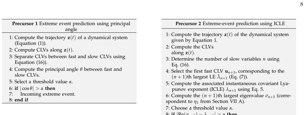
- The two precursors provide time-forecasting capability for extreme events in the tested systems.
- Critical transitions, treated as a subset of extreme events, are also predicted with the same perfect accuracy.
- The cascade-based approach applies equally to low-dimensional and higher-dimensional examples.
- Numerical evidence shows zero false positives or missed events under the tested conditions.
Where Pith is reading between the lines
- If the cascade holds more generally, the precursors could be adapted to observational time series in applications such as fluid flows or climate variables.
- Systems lacking a clear fast-slow separation might still benefit if analogous stability indicators can be defined.
- Direct comparison of the precursors against existing early-warning signals on the same benchmark systems would clarify relative strengths.
Load-bearing premise
That this specific cascade of regimes in the covariant Lyapunov vectors always occurs before extreme events in fast-slow nonlinear systems.
What would settle it
An extreme event in a fast-slow nonlinear system that occurs without the preceding slow regime of transversal tangent vectors, neutral-stability transition, and critical regime of broken transversality.
Figures


read the original abstract
We propose a theory based on dynamical systems to explain and predict the occurrence of extreme events, of which critical transitions form a subset. In fast-slow nonlinear systems, we identify a cascade of events preceding extreme events: (i) a slow regime, in which the fast covariant Lyapunov vectors (CLVs) are both tangent to the fast eigenvectors and remain transversal to the slow subspace; (ii) a transition regime, in which the fast eigenvalues become neutrally stable while the fast CLVs are no longer tangent to the fast eigenvectors; and (iii) a critical regime, in which a strong spectral gap in the eigenvalues causes both fast and slow CLVs to become tangent along the dominant fast direction, breaking the transversality between fast and slow subspaces. Building on this cascade, we propose two precursors to forewarn the occurrence of extreme events. We numerically test the theory and precursors on low- and higher-dimensional systems. The proposed precursors predict extreme events and critical transitions with 100% precision and recall. This work opens opportunities for time-forecasting extreme events using theoretically grounded precursors.
Editorial analysis
A structured set of objections, weighed in public.
Referee Report
Summary. The manuscript proposes a dynamical systems theory for extreme events (including critical transitions) in fast-slow nonlinear systems. It identifies a three-regime cascade preceding such events based on covariant Lyapunov vectors (CLVs) and eigenvalue behavior: (i) slow regime with fast CLVs tangent to fast eigenvectors yet transversal to the slow subspace; (ii) transition regime with neutral fast eigenvalues; (iii) critical regime with spectral-gap-induced tangency that breaks transversality. Two precursors are derived from this cascade and tested numerically on low- and higher-dimensional systems, with the claim that they achieve 100% precision and recall.
Significance. If the cascade proves general and the precursors robust, the work would provide a valuable theoretically grounded framework for early warning of extreme events, building on established tools like CLVs. The reported perfect performance on the tested systems is a clear strength that merits credit, as is the explicit linkage of precursors to the identified dynamical regimes rather than purely data-driven fitting.
major comments (2)
- [Abstract] Abstract: The central claim that the precursors achieve '100% precision and recall' is load-bearing for the paper's contribution, yet no information is provided on the specific systems tested (equations, dimensions, parameter values), number of extreme events, data exclusion rules, error bars, or whether the cascade and precursors were identified before or after inspecting the data. This prevents assessment of whether the perfect scores reflect genuine predictive power or post-hoc selection.
- [Numerical tests] Theory and numerical tests: The manuscript does not establish that the three-regime cascade is necessary for extreme events in fast-slow systems in general, nor does it include counter-example searches or tests under modest changes in time-scale separation or parameters. The evidence is confined to the chosen low- and higher-dimensional examples, so the universality required for the precursors to be general early-warning signals remains unproven.
minor comments (2)
- [Theory] The definition and computation of the fast and slow CLVs, including how transversality is quantified, should be stated explicitly with equations rather than assumed from prior literature.
- [Numerical tests] A brief discussion of how the precursors behave when the time-scale separation is varied continuously (rather than fixed) would strengthen the presentation.
Simulated Author's Rebuttal
We thank the referee for the constructive report and positive assessment of the work's potential significance. We address each major comment below with specific plans for revision where appropriate.
read point-by-point responses
-
Referee: [Abstract] Abstract: The central claim that the precursors achieve '100% precision and recall' is load-bearing for the paper's contribution, yet no information is provided on the specific systems tested (equations, dimensions, parameter values), number of extreme events, data exclusion rules, error bars, or whether the cascade and precursors were identified before or after inspecting the data. This prevents assessment of whether the perfect scores reflect genuine predictive power or post-hoc selection.
Authors: The full details on the tested systems (including governing equations, dimensions, and parameter values), the number of extreme events analyzed across multiple realizations, data exclusion criteria, and statistical reporting are contained in the Numerical Tests section. The cascade was derived from the covariant Lyapunov vector and eigenvalue analysis prior to any numerical validation, and the precursors follow directly from the three-regime structure rather than data-driven fitting. To make this transparent in the abstract itself, we will add a concise clause summarizing the low- and higher-dimensional examples and the scale of the tests performed. We will also ensure error bars from ensemble runs are explicitly reported in the figures and text. revision: yes
-
Referee: [Numerical tests] Theory and numerical tests: The manuscript does not establish that the three-regime cascade is necessary for extreme events in fast-slow systems in general, nor does it include counter-example searches or tests under modest changes in time-scale separation or parameters. The evidence is confined to the chosen low- and higher-dimensional examples, so the universality required for the precursors to be general early-warning signals remains unproven.
Authors: We do not claim to have proven that the cascade is necessary in every fast-slow system; the manuscript presents a dynamical mechanism observed and analyzed in representative cases, together with precursors derived from it. In the revised version we will add an explicit limitations paragraph stating the current scope, perform additional numerical checks under modest variations of the time-scale separation parameter, and include a brief search for counter-examples in systems lacking a clear spectral gap. These steps will better delineate the conditions under which the precursors are expected to apply, while acknowledging that a fully general proof lies beyond the present scope. revision: partial
Circularity Check
No significant circularity; derivation remains self-contained
full rationale
The paper's central chain proceeds from standard dynamical-systems concepts (covariant Lyapunov vectors, spectral gaps, transversality between fast/slow subspaces) to an observed cascade of regimes, then to two derived precursors whose definitions are stated explicitly in terms of those CLV and eigenvalue properties. Numerical tests on chosen low- and higher-dimensional examples are presented as validation rather than as the source of the definitions themselves; no equation or claim reduces a fitted parameter or self-citation back into the reported 100 % precision/recall figures by construction. The absence of load-bearing self-citations, ansatz smuggling, or renaming of known empirical patterns keeps the derivation independent of its own outputs.
Axiom & Free-Parameter Ledger
axioms (1)
- domain assumption Fast-slow nonlinear systems exhibit the three-regime cascade in covariant Lyapunov vectors and eigenvalues as described.
Reference graph
Works this paper leans on
-
[1]
As described in Sec- tion VIIC, in this regime, the stable CLVu st is 9 FIG
The slow regime represents the dynamics on the slow manifold, whenξ <0. As described in Sec- tion VIIC, in this regime, the stable CLVu st is 9 FIG. 5. Top: real part of the spectrum of the Jacobian in the three dynamical regimes: the slow regime, the transition regime, and the critical regime. In blue, green, and red the fast eigenvalues, and in black th...
-
[2]
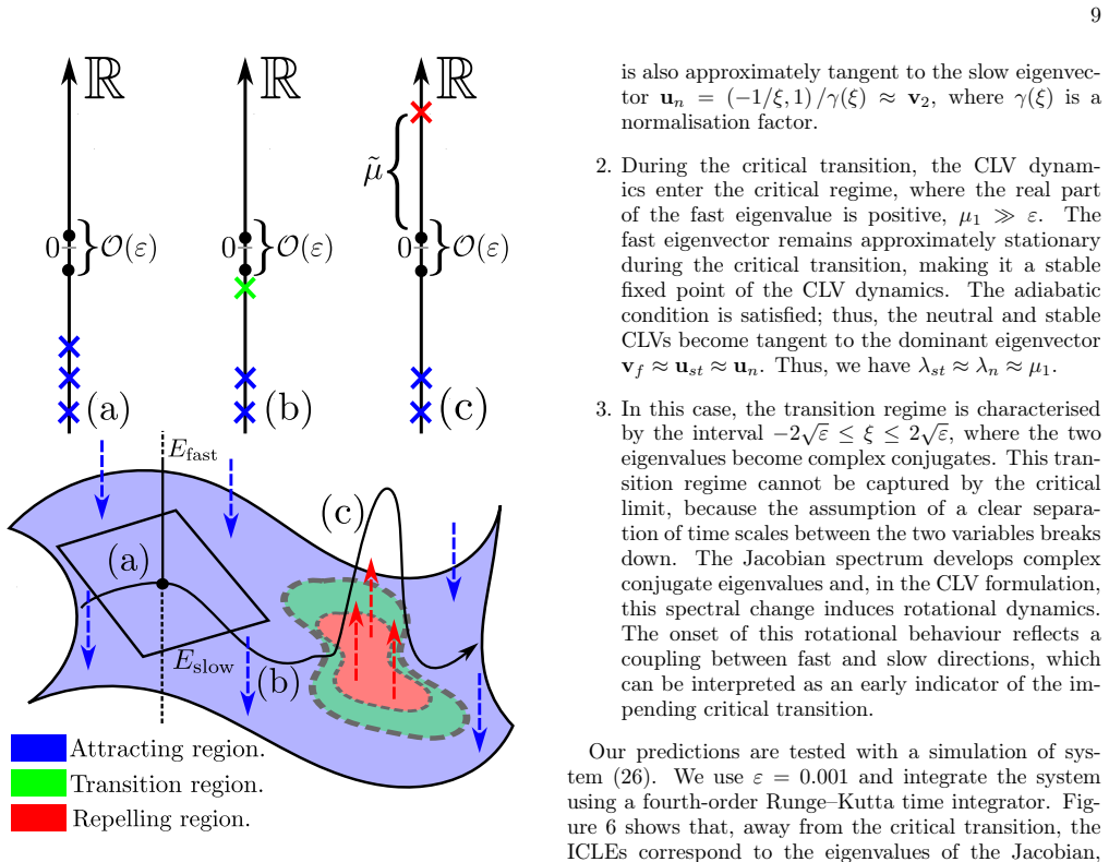
The fast eigenvector remains approximately stationary during the critical transition, making it a stable fixed point of the CLV dynamics
During the critical transition, the CLV dynam- ics enter the critical regime, where the real part of the fast eigenvalue is positive,µ 1 ≫ε. The fast eigenvector remains approximately stationary during the critical transition, making it a stable fixed point of the CLV dynamics. The adiabatic condition is satisfied; thus, the neutral and stable CLVs become...
-
[3]
low temperature
In this case, the transition regime is characterised by the interval−2 √ε≤ξ≤2 √ε, where the two eigenvalues become complex conjugates. This tran- sition regime cannot be captured by the critical limit, because the assumption of a clear separa- tion of time scales between the two variables breaks down. The Jacobian spectrum develops complex conjugate eigen...
-
[4]
Farazmand and T
M. Farazmand and T. P. Sapsis, Applied Mechanics Re- views71, 050801 (2019)
2019
-
[5]
M. Ghil, P. Yiou, S. Hallegatte, B. D. Malamud, P. Naveau, A. Soloviev, P. Friederichs, V. Keilis-Borok, D. Kondrashov, V. Kossobokov, O. Mestre, C. Nicolis, H. W. Rust, P. Shebalin, M. Vrac, A. Witt, and I. Zali- apin, Nonlinear Processes in Geophysics18, 295 (2011)
2011
-
[6]
C. F. Ropelewski and M. S. Halpert, Monthly Weather Review115, 1606 (1987)
1987
-
[7]
D. R. Easterling, J. L. Evans, P. Ya. Groisman, T. R. Karl, K. E. Kunkel, and P. Ambenje, Bulletin of the American Meteorological Society81, 417 (2000)
2000
-
[8]
Dysthe, H
K. Dysthe, H. E. Krogstad, and P. Müller, Annual Re- view of Fluid Mechanics40, 287 (2008)
2008
-
[9]
D. R. Solli, C. Ropers, P. Koonath, and B. Jalali, Nature 450, 1054 (2007)
2007
-
[10]
T. P. Sapsis, Annual Review of Fluid Mechanics53, 85 (2021)
2021
-
[11]
P. K. Yeung, X. M. Zhai, and K. R. Sreenivasan, Pro- ceedings of the National Academy of Sciences112, 12633 (2015). 15 TABLE II. Comparison of algorithms across dynamical systems. Bistable Rössler FitzHugh–NagumoMultiscale Lorenz 96 Precursor 1 F-score = 1 NA F-score = 0.99 Precursor 2 F-score = 1 F-score = 1 F-score = 1
2015
-
[12]
P. J. Blonigan, M. Farazmand, and T. P. Sapsis, Physical Review Fluids4, 044606 (2019)
2019
-
[14]
X. Fang, S. Misra, G. Xue, and D. Yang, IEEE Commu- nications Surveys & Tutorials14, 944 (2012)
2012
-
[15]
Huhn and L
F. Huhn and L. Magri, Journal of Fluid Mechanics882, A24 (2020)
2020
-
[16]
Scheffer, J
M. Scheffer, J. Bascompte, W. A. Brock, V. Brovkin, S.R.Carpenter, V.Dakos, H.Held, E.H.vanNes, M.Ri- etkerk, and G. Sugihara, Nature461, 53 (2009)
2009
-
[17]
Scheffer, S
M. Scheffer, S. R. Carpenter, T. M. Lenton, J. Bas- compte, W. Brock, V. Dakos, J. van de Koppel, I. A. van de Leemput, S. A. Levin, E. H. van Nes, M. Pascual, and J. Vandermeer, Science338, 344 (2012)
2012
-
[18]
Kuehn, Physica D: Nonlinear Phenomena240, 1020 (2011)
C. Kuehn, Physica D: Nonlinear Phenomena240, 1020 (2011)
2011
-
[19]
Kuehn,Multiple Time Scale Dynamics, Vol
C. Kuehn,Multiple Time Scale Dynamics, Vol. 191 (Springer, 2015)
2015
-
[20]
Dakos, M
V. Dakos, M. Scheffer, E. H. van Nes, V. Brovkin, V. Petoukhov, and H. Held, Proceedings of the National Academy of Sciences105, 14308 (2008)
2008
-
[21]
Qi and A
D. Qi and A. J. Majda, Proceedings of the National Academy of Sciences117, 52 (2020)
2020
-
[22]
N. A. K. Doan, W. Polifke, and L. Magri, Proceedings of the Royal Society A: Mathematical, Physical and Engi- neering Sciences477(2021)
2021
-
[23]
Racca and L
A. Racca and L. Magri, Physical Review Fluids7, 104402 (2022)
2022
-
[24]
Faranda, G
D. Faranda, G. Messori, and P. Yiou, Scientific Reports 7, 41278 (2017)
2017
-
[25]
Martín, J
D. Martín, J. Grau, and L. Jofre, Scientific Reports15, 29629 (2025)
2025
-
[26]
O. T. Schmidt and P. J. Schmid, Journal of Fluid Me- chanics867, R2 (2019)
2019
-
[27]
Madhusudanan and R
A. Madhusudanan and R. R. Kerswell, Journal of Fluid Mechanics1003, A5 (2025)
2025
-
[28]
Farazmand and T
M. Farazmand and T. P. Sapsis, Science Advances3, e1701533 (2017)
2017
-
[29]
Pickering, S
E. Pickering, S. Guth, G. E. Karniadakis, and T. P. Sap- sis, Nature Computational Science2, 823 (2022)
2022
-
[31]
A. J. Fox, Physical Review Fluids8, 10.1103/Phys- RevFluids.8.094401 (2023)
-
[32]
M. W. Beims and J. A. C. Gallas, Scientific Reports6, 37102 (2016)
2016
-
[33]
Sharafi, M
N. Sharafi, M. Timme, and S. Hallerberg, Physical Re- view E96, 032220 (2017)
2017
-
[34]
Ruelle, Publications Mathématiques de l’Institut des Hautes Études Scientifiques50, 27 (1979)
D. Ruelle, Publications Mathématiques de l’Institut des Hautes Études Scientifiques50, 27 (1979)
1979
-
[35]
Ginelli, H
F. Ginelli, H. Chaté, R. Livi, and A. Politi, Journal of Physics A: Mathematical and Theoretical46, 254005 (2013)
2013
-
[36]
P. V. Kuptsov and U. Parlitz, Journal of Nonlinear Sci- ence22, 727 (2012)
2012
-
[37]
Pikovsky and A
A. Pikovsky and A. Politi,Lyapunov Exponents: A Tool to Explore Complex Dynamics(Cambridge University Press, 2016)
2016
-
[38]
H.-l. Yang, K. A. Takeuchi, F. Ginelli, H. Chaté, and G. Radons, Physical Review Letters102, 074102 (2009)
2009
-
[39]
H.-l. Yang, G. Radons, and H. Kantz, Physical Review Letters109, 244101 (2012)
2012
-
[40]
X. Ding, H. Chaté, P. Cvitanović, E. Siminos, and K. A. Takeuchi, Physical Review Letters117, 024101 (2016)
2016
-
[41]
P. V. Kuptsov and S. P. Kuznetsov, Regular and Chaotic Dynamics23, 908 (2018)
2018
-
[42]
Ginelli, P
F. Ginelli, P. Poggi, A. Turchi, H. Chaté, R. Livi, and A. Politi, Physical Review Letters99, 130601 (2007)
2007
-
[43]
C. L. Wolfe and R. M. Samelson, Tellus A59, 355 (2007)
2007
-
[44]
Froyland, T
G. Froyland, T. Hüls, G. P. Morriss, and T. M. Watson, Physica D: Nonlinear Phenomena247, 18 (2013)
2013
-
[45]
F. X. Moreira Huhn,Optimisation of Chaotic Thermoa- coustics, Ph.D. thesis, Apollo - University of Cambridge Repository (2021)
2021
-
[46]
Margazoglou and L
G. Margazoglou and L. Magri, Nonlinear Dynamics111, 8799 (2023)
2023
-
[47]
Özalp, G
E. Özalp, G. Margazoglou, and L. Magri, Chaos: An Interdisciplinary Journal of Nonlinear Science33, 093107 (2023)
2023
-
[48]
Özalp and L
E. Özalp and L. Magri, Nonlinear Dynamics113, 13791 (2025)
2025
- [49]
-
[50]
Eckmann and O
J.-P. Eckmann and O. Gat, Journal of Statistical Physics 98, 775 (2000)
2000
-
[51]
M.Carlu, F.Ginelli, V.Lucarini,andA.Politi,Nonlinear Processes in Geophysics26, 73 (2019)
2019
-
[52]
Martin, N
C. Martin, N. Sharafi, and S. Hallerberg, Chaos: An In- terdisciplinary Journal of Nonlinear Science32, 033105 (2022)
2022
-
[53]
E. L. Brugnago, J. A. C. Gallas, and M. W. Beims, Chaos: An Interdisciplinary Journal of Nonlinear Science 30, 083106 (2020)
2020
-
[54]
Viennet, N
A. Viennet, N. Vercauteren, M. Engel, and D. Faranda, Chaos: An Interdisciplinary Journal of Nonlinear Science 32, 113145 (2022)
2022
-
[55]
Babaee and T
H. Babaee and T. P. Sapsis, Proceedings of the Royal Society A: Mathematical, Physical and Engineering Sci- ences472, 20150779 (2016)
2016
-
[56]
Farazmand and T
M. Farazmand and T. P. Sapsis, Physical Review E94, 032212 (2016)
2016
-
[57]
A. Blanchard and T. P. Sapsis, SIAM Journal on Applied Dynamical Systems18, 1143 (2019), https://doi.org/10.1137/18M1212082
-
[58]
C. Pugh, M. Shub, and a. a. b. A. Starkov, Bulletin of the American Mathematical Society41, 1 (2004)
2004
-
[59]
Bochi and M
J. Bochi and M. Viana, Annals of Mathematics161, 1423 (2005). 16
2005
-
[60]
V. I. Arnold,Ordinary Differential Equations(Springer Science & Business Media, 1992)
1992
-
[61]
V. I. Oseledets, Trudy Moskovskogo Matematicheskogo Obshchestva19, 179 (1968), english translation inTrans- actions of the Moscow Mathematical Society, 19 (1968), 197–231
1968
-
[62]
P. V. Kuptsov, Physical Review E85, 015203 (2012)
2012
-
[63]
In this section, we drop the subscriptifor brevity
-
[64]
Writingδuin the Jacobian eigenbasis givesJδu=VΛa, whereV,Λ, andaare generally complex
The vectorJδuis real because both the JacobianJand the perturbationδuare real. Writingδuin the Jacobian eigenbasis givesJδu=VΛa, whereV,Λ, andaare generally complex. However, sinceJis real, these com- plex quantities occur in conjugate pairs, so the imaginary parts cancel andJδuremains real
-
[65]
Fenichel, Journal of Differential Equations31, 53 (1979)
N. Fenichel, Journal of Differential Equations31, 53 (1979)
1979
-
[66]
O. E. Rössler, Zeitschrift für Naturforschung A38, 788 (1983)
1983
-
[67]
G. Ansmann, K. Rajat, K. Lehnertz, and U. Feudel, Physical Review E88, 10.1103/PhysRevE.88.052911 (2013)
-
[68]
E. N. Lorenz, inSeminar on Predictability, Vol. 1 (Eu- ropean Centre for Medium-Range Weather Forecasts (ECMWF), Reading, United Kingdom, 1995) pp. 1–18
1995
discussion (0)
Sign in with ORCID, Apple, or X to comment. Anyone can read and Pith papers without signing in.