Recognition: unknown
Breakdown of the Migdal-Eliashberg theory for electron-phonon systems. Role of polarons/bi-polarons
Pith reviewed 2026-05-10 12:08 UTC · model grok-4.3
The pith
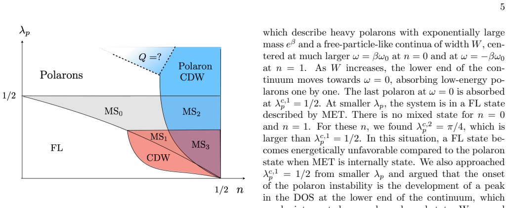
Migdal-Eliashberg theory collapses to polaron states at couplings below phonon softening
A machine-rendered reading of the paper's core claim, the machinery that carries it, and where it could break.
Core claim
Using variational considerations we establish rigorous upper bounds on the coupling λ at which a Fermi liquid state transforms into the bipolaron/polaron state. We show that at small and near-maximum densities this happens well before a dressed phonon softens. This is true both in 2D and 3D systems; in the latter the upper bound on λ tends to zero in the limit of small or near-full density. Polaron formation is produced by fermions with energies comparable to the bandwidth and thus lies outside the realm of Migdal-Eliashberg theory.
What carries the argument
Variational upper bounds on the energy that identify the coupling strength where the polaron or bipolaron state becomes energetically favorable over the Fermi liquid.
If this is right
- At low and high densities the polaron/bipolaron instability precedes phonon softening.
- In 3D the critical λ bound vanishes at extreme densities.
- Near half filling a charge-density-wave state appears first.
- A strong-coupling regime of Migdal-Eliashberg theory exists near the CDW instability before polaron formation.
Where Pith is reading between the lines
- This breakdown mechanism suggests that low-density materials may show polaronic behavior at moderate couplings without phonon softening.
- The variational approach could be applied to other electron-boson models to find similar early instabilities.
- Direct simulations at intermediate densities would map the full phase diagram between the variational bounds and exact results.
Load-bearing premise
Variational upper bounds on energy reliably identify the first instability to polaron/bipolaron states for generic densities without a lower-energy competing state existing between the Fermi liquid and polaron regimes.
What would settle it
A numerical calculation of the Holstein model ground state at low density that remains Fermi-liquid-like with finite phonon frequency up to a λ larger than the reported variational upper bound.
Figures


read the original abstract
The Migdal-Eliashberg theory (MET) describes electrons interacting with phonons in the adiabatic limit when the phonon Debye frequency is much smaller than the Fermi energy. A conventional belief is that MET holds even at strong coupling, when electron self-energy is large, and breaks down only near the point where the dressed phonon spectrum softens to near zero. We analyze numerically and analytically a different option -- collapse to a polaronic/bipolaronic ground state. The last scenario has never been analyzed in precise quantitative terms for a generic electron density. Using variational considerations, we establish rigorous upper bounds on the coupling $\lambda$, at which a FL state transforms into the bipolaron/polaron state. We show that at small and near-maximum densities, this happens well before a dressed phonon softens. This is true both in 2D and 3D systems; in the latter the upper bound on $\lambda$ tends to zero in the limit of small or near-full density. We present analytical reasoning for this behavior based on hints extracted from exact diagrammatic treatment of the on-site Holstein model for the spin polarized case and argue that polarons are produced by fermions with energies comparable to the bandwidth; i.e., polaron formation is outside the realm of MET. Closer to half-filling, the leading instability upon increasing $\lambda$ is towards a charge-density-wave state (CDW), and there exists a strong coupling regime of MET near this instability, while the polaron/bipolaron state develops at larger $\lambda$ out of a CDW-ordered state and inherits a CDW order over some range of coupling.
Editorial analysis
A structured set of objections, weighed in public.
Referee Report
Summary. The manuscript claims that Migdal-Eliashberg theory (MET) for electron-phonon systems breaks down at strong coupling via a transition to a polaronic/bipolaronic ground state before the dressed phonon softens, at least at small and near-maximum densities. Variational considerations are used to derive rigorous upper bounds on the coupling λ for the Fermi-liquid to polaron/bipolaron transformation in both 2D and 3D; these bounds lie below the softening point. Near half-filling the leading instability is instead a charge-density-wave (CDW) state, with the polaron state appearing at larger λ out of the CDW phase. Analytical support is drawn from exact diagrammatic results on the spin-polarized Holstein model.
Significance. If the central claim holds, the work supplies concrete, falsifiable upper bounds on the regime of MET validity and clarifies that polaron formation can preempt phonon softening outside the adiabatic, low-energy window assumed by MET. The variational upper-bound technique and the link to exact Holstein-model diagrammatics are genuine strengths that make the bounds rigorous and reproducible in principle.
major comments (2)
- [Variational considerations and low-density analysis] The identification of the polaron/bipolaron state as the first instability (rather than a competing ordered phase) rests on the variational ansatz being globally optimal. While the manuscript correctly notes CDW dominance near half-filling, the low-density regime relies on Holstein-model hints without explicit energy comparisons between the polaron variational wavefunction and alternative states (e.g., modulated CDW or other density-wave ansätze) at the same λ and n. This comparison is load-bearing for the claim that MET breaks down specifically because of polarons.
- [3D systems near small or full density] In the 3D small- and near-full-density limits the upper bound on λ is stated to tend to zero. The derivation of this limit and the explicit demonstration that the corresponding phonon-softening λ remains finite should be shown in a dedicated subsection or appendix, including the functional form of the variational energy as density approaches the band edge.
minor comments (2)
- [Abstract] The abstract states that the analysis is performed 'numerically and analytically,' yet the quantitative results presented appear to be dominated by variational bounds and Holstein diagrammatics. A brief clarification of the numerical methods (e.g., exact diagonalization or Monte Carlo parameters) and their error bars would improve reproducibility.
- [Notation and definitions] Notation for the dimensionless coupling λ, the density n, and the variational parameters should be collected in a single table or early section to aid readers.
Simulated Author's Rebuttal
We thank the referee for the careful reading, positive assessment of the significance, and constructive suggestions. We address the two major comments point by point below. We will revise the manuscript to incorporate clarifications and additional derivations where needed.
read point-by-point responses
-
Referee: [Variational considerations and low-density analysis] The identification of the polaron/bipolaron state as the first instability (rather than a competing ordered phase) rests on the variational ansatz being globally optimal. While the manuscript correctly notes CDW dominance near half-filling, the low-density regime relies on Holstein-model hints without explicit energy comparisons between the polaron variational wavefunction and alternative states (e.g., modulated CDW or other density-wave ansätze) at the same λ and n. This comparison is load-bearing for the claim that MET breaks down specifically because of polarons.
Authors: We agree that an explicit energy comparison to possible competing ordered states would further strengthen the low-density claim. At low densities the Fermi surface lacks the nesting vectors required for a modulated CDW instability (as already indicated by the exact diagrammatic results on the spin-polarized Holstein model that we cite). The variational upper bound we derive is nevertheless rigorous: it shows that the polaron/bipolaron energy lies below the FL energy at a value of λ strictly smaller than the phonon-softening point, independent of whether other instabilities exist. In the revision we will add a short paragraph in the low-density section that explicitly contrasts the variational polaron energy with the expected cost of a modulated CDW at the same n and λ, using the Holstein-model insights already present in the manuscript. revision: partial
-
Referee: [3D systems near small or full density] In the 3D small- and near-full-density limits the upper bound on λ is stated to tend to zero. The derivation of this limit and the explicit demonstration that the corresponding phonon-softening λ remains finite should be shown in a dedicated subsection or appendix, including the functional form of the variational energy as density approaches the band edge.
Authors: We accept the suggestion. In the revised manuscript we will add a dedicated appendix that derives the vanishing of the variational upper bound on λ as n → 0 or n → 1 in three dimensions. The appendix will expand the variational energy functional near the band edge, demonstrate that the critical λ for polaron formation approaches zero, and contrast this with the phonon-softening λ of MET, which remains finite because it is controlled by the density of states at the Fermi level (which stays nonzero away from the exact band edge). revision: yes
Circularity Check
No significant circularity; derivation relies on standard variational bounds and independent diagrammatics.
full rationale
The paper's central result uses variational wavefunctions to obtain rigorous upper bounds on the critical coupling λ where the polaron/bipolaron energy falls below the Fermi-liquid energy. This is a standard, non-circular application of the variational principle: the computed variational energy provides an upper bound on the true ground-state energy without defining the target instability in terms of itself. The comparison to the phonon-softening point from Migdal-Eliashberg theory or diagrammatic calculations is external to the variational step. References to prior exact treatments of the Holstein model supply supporting hints but do not carry the load-bearing argument; the variational bounds stand on their own and are falsifiable by direct energy minimization. No parameters are fitted and then relabeled as predictions, no ansatz is smuggled via self-citation, and no uniqueness theorem is invoked to force the result. The derivation chain is therefore self-contained.
Axiom & Free-Parameter Ledger
axioms (2)
- domain assumption Adiabatic limit where phonon Debye frequency is much smaller than Fermi energy
- standard math Variational methods provide rigorous upper bounds on ground-state energies for state comparison
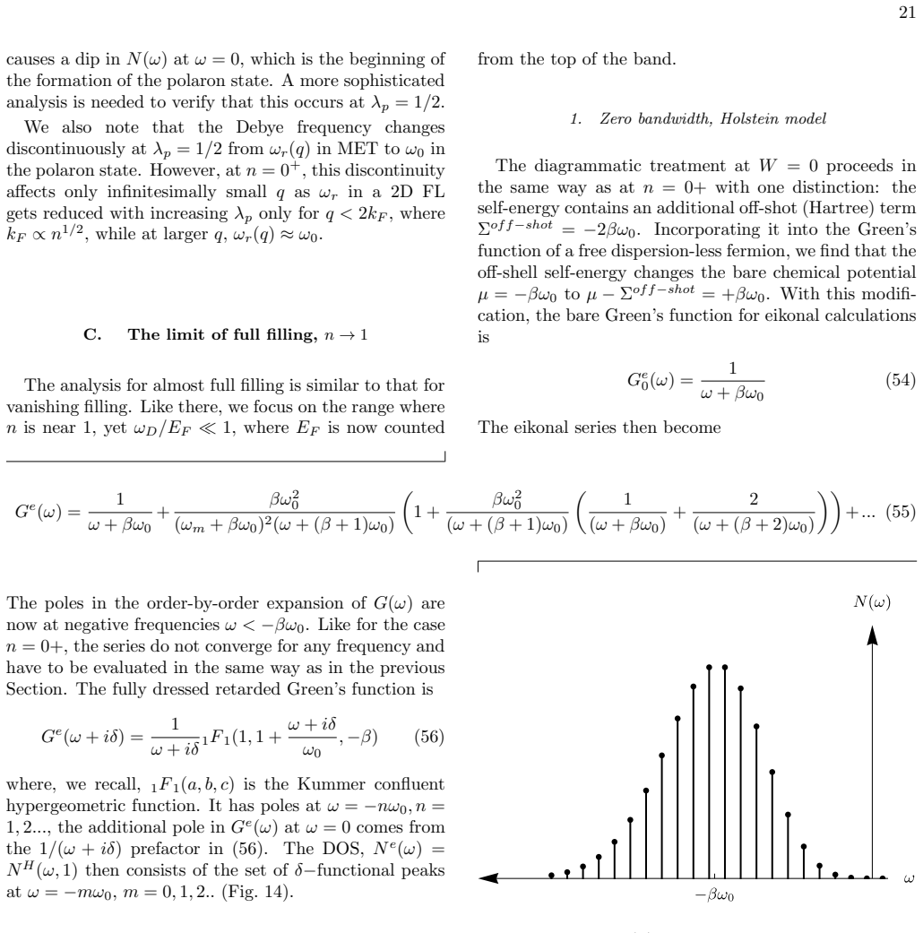
Forward citations
Cited by 1 Pith paper
-
Apparent Planckian scattering from local polaron formation
Local polaron formation in the disordered Holstein model generates apparent Planckian scattering Γ_tr = Γ0 + α k_B T / ℏ with α ~ O(1) from quasielastic scattering, as evidenced by Monte Carlo simulations.
Reference graph
Works this paper leans on
-
[1]
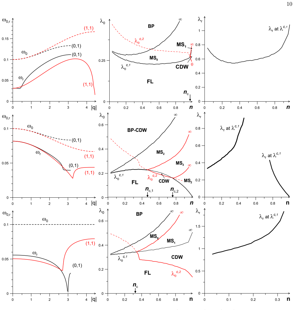
3D case The 3D phase diagram, obtained in the variational study for dispersion-lessω 0 and spin-full fermions, is pre- sented in the middle of the lower panel in Fig. 4. For convenience, in Fig.31 we re-plot this phase diagram in units ofλ p and for spin-less fermions. We note that phase diagrams in 2D and 3D are similar, but there is one key distinction:...
-
[2]
Finite T At temperatures above any ordering transition, the evolution from the FL state to the polaron state is smooth. Nevertheless, numerical calculations have shown that this crossover occurs rapidly [27, 68, 70, 72, 74, 75, 78, 79], and can be identified by the onset of a pseudo- gap in the electronic density of states [70]. As detailed in Sec.IV D 2,...
-
[3]
andN F = (2/πW). This self- energy can be split into static and dynamic parts: Σ(1)(ωm) = Σ(1)(0) + Σ(1) dyn(ωm) (A3) where Σ(1)(0) =−λ 0ω0 log W ω0 , Σ(1) dyn(ωm) =−λ 0ω0 log ω0 ω0 −iω m ,(A4) The first term, which depends onW, accounts for the renormalization of the chemical potential,µ=µ 0 − Σ(1)(0), and the second, which does not depend on W, is respo...
-
[4]
Both containλ 2 0 in the prefactors, and in the calculations to this order, the renormalization ofµ 0 into µcan be neglected
Combining it with the O(λ0) contribution and expanding inω m, we obtain: Σ(1) dyn(ωm) =−iλ 0ωm +iλ 2 0ωm log W ω0 (A5) We now compute the two two-loop self-energies, Σ (2v) and Σ(2r). Both containλ 2 0 in the prefactors, and in the calculations to this order, the renormalization ofµ 0 into µcan be neglected. We start with the vertex correc- tion diagram, ...
-
[5]
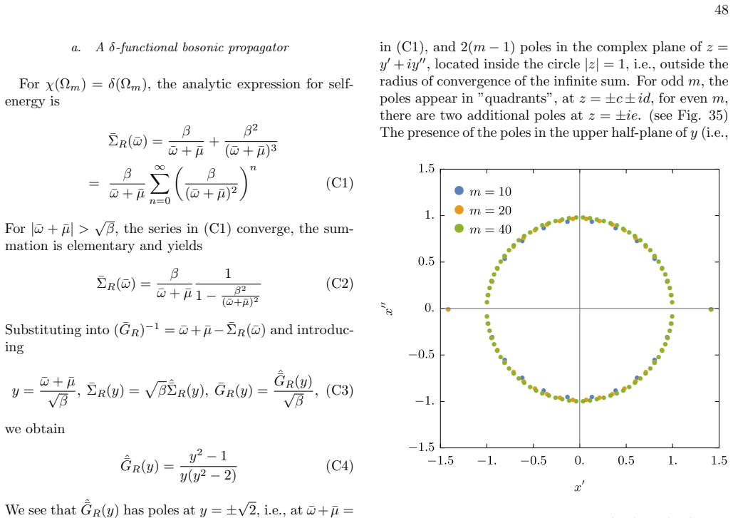
Rainbow approximation We writeG −1 R (ω) =ω+µ−Σ R(ω), where the subindex indicates that we compute the self-energy by keeping only rainbow diagrams (one diagram at each loop order), see Fig. 34. We measureω,µand Σ R in units ofω 0 and introduce ¯ω=ω/ω 0, ¯µ=µ/ω 0 and ¯ΣR = Σ R/ω0. For the Green’s function, we introduce ¯GR =G R ω0. 48 a. Aδ-functional bos...
-
[6]
(C12) where, we recall, ¯ω=ω/ω 0 and ¯µ=µ/ω0
the rainbow series yields ¯ΣR(¯ω) = β ¯ω+ ¯µ−1+ β2 (¯ω+ ¯µ−1)2(¯ω+ ¯µ−2)+.... (C12) where, we recall, ¯ω=ω/ω 0 and ¯µ=µ/ω0. Eq. (C12) be re-expressed in terms ofx= ¯ω+ ¯µas ¯ΣR(x, β) = ∞X n=1 βn x−n n−1Y m=1 1 (x−m) !2 = ∞X n=1 βn x−n 1 ((1−x) n−1)2 (C13) where (a) b is a Pochhammer function. The sum con- verges for all non-integerxand diverges quadratica...
-
[7]
We show the corresponding diagrams in Fig
Self-consistent one-loop approximation We now extend the perturbation series to include all renormalizations of the internal fermionic propagator in the self-energy diagram , e.g., two subsequent rainbow renormalizations. We show the corresponding diagrams in Fig. 40. The sum of the diagrammatic series can be formally represented in a compact form by repl...
-
[8]
we again usex= ˜ω+ ˜µ. The perturbation series for the self-energy yield ¯Σ1L(x, β) = β x−1 + β2 (x−1) 2(x−2) + β3 (x−1) 2(x−2) 2 1 (x−3) + 1 x−1 + β4 (x−1) 2(x−2) 2 1 (x−3) 2(x−4) + 1 (x−2)(x−3) 2 + 2 (x−1)(x−2)(x−3) + 1 (x−1) 2(x−2) +...(C29) As before, we introduce a partial sum ofmterms, ¯Σ(m) 1L (x, β) and analyze the poles of ¯G(m) 1L (z, β) in the ...
-
[9]
We recall that eikonal calculation reproduces the exact Green’s function of the Holstein model at zero density
Comparison with the eikonal calculation We now compare the results of the rainbow and self- consistent one-loop approximations, which both neglect vertex corrections, with the Green’s function that we obtained in the main text using the eikonal computa- tional technique which includes vertex corrections on equal footings with the renormalization of the pr...
-
[10]
The known results Lang-Firsov transformation is a convenient way to di- agonalize the single-site Holstein HamiltonianH: H=ω 0 X i a† i ai + p βω0 X i c† i ci(ai +a † i) (E1) We consider the Hamiltonian here and do not add the chemical potentialµ. Lang and Firsov demonstrated that this Hamiltonian can be exactly diagonalized via the uni- tary transformati...
-
[11]
To do this, we evalu- ate the off-diagonal elements of the dressed hopping op- erator ˜V= P i,j tijc† i cjX † i Xj
Our results We compute the damping rate of fermions in patchm due to transitions to other patches. To do this, we evalu- ate the off-diagonal elements of the dressed hopping op- erator ˜V= P i,j tijc† i cjX † i Xj. From physics perspective, these terms describe incoherent scattering processes in which a polaron changes its momentum and patch num- ber, lea...
-
[12]
Devreese, Electron–phonon interac- tions and the response of polarons, in Encyclopedia of Condensed Matter Physics, edited by F
J. Devreese, Electron–phonon interac- tions and the response of polarons, in Encyclopedia of Condensed Matter Physics, edited by F. Bassani, G. L. Liedl, and P. Wyder (Elsevier, Oxford, 2005) pp. 99–109
2005
-
[13]
Aleksandrov and J
A. Aleksandrov and J. Derreese, Advances in Polaron Physics (Springer Berlin Hei- delberg, Springer-Verlag, Berlin Heidelberg, 2010)
2010
-
[14]
Franchini, M
C. Franchini, M. Reticcioli, M. Setvin, and U. Diebold, Polarons in materials, Nature Reviews Materials6, 560 (2021)
2021
- [15]
-
[16]
A. B. Migdal, Interactions between electrons and lattice vibrations in a superconductor, Sov. Phys. JETP7, 996 (1958)
1958
-
[17]
G. M. Eliashberg, Interactions between electrons and lat- tice vibrations in a superconductor, JETP11, 696 (1960)
1960
-
[18]
A. A. Abrikosov, L. P. Gorkov, and I. E. Dzyaloshinski, Methods of Quantum Feld Theory in Statistical Physics (Pergamon Oxford, 1965)
1965
-
[19]
O. V. Dolgov, I. I. Mazin, A. A. Golubov, S. Y. Savrasov, and E. G. Maksimov, Critical temperature and enhanced isotope effect in the presence of paramagnons in phonon- mediated superconductors, Phys. Rev. Lett.95, 257003 (2005); Y. Wang and A. Chubukov, Quantum-critical pairing in electron-doped cuprates, Phys. Rev. B88, 024516 (2013)
2005
-
[20]
A. V. Chubukov, A. Abanov, I. Esterlis, and S. A. Kivel- son, Eliashberg theory of phonon-mediated superconduc- tivity – when it is valid and how it breaks down, Annals of Physics417, 168190 (2020)
2020
-
[21]
Mirabi, R
S. Mirabi, R. Boyack, and F. Marsiglio, Thermodynam- ics of eliashberg theory in the weak-coupling limit, Phys. Rev. B102, 214505 (2020)
2020
-
[22]
M. K.-H. Kiessling, B. L. Altshuler, and E. A. Yuzbashyan, Bounds on$$t c$$in the eliashberg theory of superconductivity. ii: Dispersive phonons, Journal of Statistical Physics192, 94 (2025); Bounds on$$t c$$in the eliashberg theory of superconductivity. iii: Einstein phonons,192, 93 (2025); N. V. Gnezdilov and R. Boyack, Upper bound ont c in a strongly c...
-
[23]
At weak coupling,λ≪1, EliashbergT c = 1.13√eω0e−1/λ = 0.69ωe−1/λ, whereω 0 is the Debye fre- quency (see [? ?] and references therein), which differs 62 by √efrom the often cited value 1.13, which holds for the case when the phonon susceptibility is set to be constant at frequencies smaller thanω 0 and zero otherwise
-
[24]
E. A. Yuzbashyan, B. L. Altshuler, and A. Patra, Insta- bility of metals with respect to strong electron-phonon interaction, Phys. Rev. Lett.135, 026503 (2025); E. A. Yuzbashyan and B. L. Altshuler, Breakdown of the migdal-eliashberg theory and a theory of lattice-fermionic superfluidity, Phys. Rev. B106, 054518 (2022); Migdal- eliashberg theory as a clas...
2025
-
[25]
A. S. Alexandrov, V. V. Kabanov, and D. K. Ray, From electron to small polaron: An exact cluster solution, Phys. Rev. B49, 9915 (1994)
1994
-
[26]
A. S. Alexandrov and N. F. Mott, Bipolarons, Reports on Progress in Physics57, 1197 (1994); Polarons and Bipolarons (WORLD SCIENTIFIC, 1996) https://www.worldscientific.com/doi/pdf/10.1142/2784
-
[27]
G. D. Mahan, Many-Particle Physics, 3rd ed., Physics of Solids and Liquids (Kluwer Academic/Plenum Publish- ers, New York, 2000)
2000
-
[28]
We emphasize that vertex corrections are still small in this regime, asω r(q) is smaller thanE F for allq. In this respect strong coupling MET for electron-phonon inter- action is different from an effective MET for electrons interacting with soft fluctuations in spin or charge chan- nel (see Refs. [22] for more details)
-
[29]
Combescot, Strong-coupling limit of eliashberg theory, Phys
R. Combescot, Strong-coupling limit of eliashberg theory, Phys. Rev. B51, 11625 (1995)
1995
-
[30]
Wu, S.-S
Y.-M. Wu, S.-S. Zhang, A. Abanov, and A. V. Chubukov, Interplay between superconductivity and non-fermi liq- uid at a quantum critical point in a metal. v. theγmodel and its phase diagram. the caseγ= 2, Phys. Rev. B103, 024522 (2021)
2021
-
[31]
B. K. Chakraverty, J. Ranninger, and D. Feinberg, Ex- perimental and theoretical constraints of bipolaronic su- perconductivity in highT c materials: An impossibility, Phys. Rev. Lett.81, 433 (1998)
1998
-
[32]
B. K. Chakraverty, J. Ranninger, and D. Feinberg, Chakraverty et al. reply:, Phys. Rev. Lett.82, 2621 (1999)
1999
-
[33]
Zhang, E
S.-S. Zhang, E. Berg, and A. V. Chubukov, Free en- ergy and specific heat near a quantum critical point of a metal, Phys. Rev. B107, 144507 (2023); S.-S. Zhang, Z. M. Raines, and A. V. Chubukov, Applicabil- ity of eliashberg theory for systems with electron-phonon and electron-electron interaction: A comparative analy- sis,109, 245132 (2024)
2023
-
[34]
Abanov and A
A. Abanov and A. V. Chubukov, Interplay between su- perconductivity and non-Fermi liquid at a quantum criti- cal point in a metal. i. theγmodel and its phase diagram atT= 0: The case 0< γ <1, Phys. Rev. B102, 024524 (2020)
2020
-
[35]
Marsiglio, Eliashberg theory: A short review, Annals of Physics417, 168102 (2020)
F. Marsiglio, Eliashberg theory: A short review, Annals of Physics417, 168102 (2020)
2020
-
[36]
Lang and Y
I. Lang and Y. A. Firsov, Kinetic theory of semiconduc- tors with low mobility, JETP16, 1301 (1963)
1963
-
[37]
Holstein, Studies of polaron motion: Part i
T. Holstein, Studies of polaron motion: Part i. the molecular-crystal model, Annals of Physics8, 325 (1959)
1959
-
[38]
Ranninger, Spectral properties of small-polaron sys- tems, Phys
J. Ranninger, Spectral properties of small-polaron sys- tems, Phys. Rev. B48, 13166 (1993)
1993
-
[39]
N. V. Prokof’ev and B. V. Svistunov, Polaron problem by diagrammatic quantum monte carlo, Phys. Rev. Lett. 81, 2514 (1998)
1998
-
[40]
A. S. Mishchenko, N. V. Prokof’ev, A. Sakamoto, and B. V. Svistunov, Diagrammatic quantum monte carlo study of the fr¨ ohlich polaron, Phys. Rev. B62, 6317 (2000)
2000
-
[41]
V., Diagrammatics (World Scientific Pub- lishing Co (2006), 2006)
Sadovskii, M. V., Diagrammatics (World Scientific Pub- lishing Co (2006), 2006)
2006
-
[42]
E. Z. Kuchinskiy and M. V. Sadovskiy, Generalized dy- namical keldysh model, Journal of Experimental and Theoretical Physics166, 45–62 (2024)
2024
-
[43]
L´ evy and J
M. L´ evy and J. Sucher, Eikonal approximation in quan- tum field theory, Phys. Rev.186, 1656 (1969)
1969
-
[44]
P. A. Lee, T. M. Rice, and P. W. Anderson, Fluctuation effects at a peierls transition, Phys. Rev. Lett.31, 462 (1973)
1973
-
[45]
A. L. Efros, Theory of electron states in heavily doped semiconductors, Sov. Phys. JETP32, 479 (1971)
1971
-
[46]
M. V. Sadovskii, A model of a disordered system (a con- tribution to the theory of ”liquid semiconductors”), Sov. Phys. JETP39, 845 (1974)
1974
-
[47]
Posazhennikova and P
A. Posazhennikova and P. Coleman, Quenched disorder formulation of the pseudogap problem, Phys. Rev. B67, 165109 (2003)
2003
-
[48]
M. N. Kiselev and K. A. Kikoin, Scalar and vector keldysh models in the time domain, JETP Letters89, 114 (2009); D. V. Efremov and M. N. Kiselev, Seven ´Etudes on dynamical Keldysh model, SciPost Phys. Lect. Notes , 65 (2022)
2009
-
[49]
M. V. Sadovskii, Theory of quasi-one-dimensional sys- tems undergoing a peierls transition, Sov. Phys. – Solid State16, 1632 (1974)
1974
-
[50]
Tchernyshyov, Pseudogap in one dimension, Phys
O. Tchernyshyov, Pseudogap in one dimension, Phys. Rev. B59, 1358 (1999)
1999
-
[51]
Yamase and W
H. Yamase and W. Metzner, Fermi-surface truncation from thermal nematic fluctuations, Phys. Rev. Lett.108, 186405 (2012)
2012
-
[52]
Vilk and A.-M.S
Y.M. Vilk and A.-M.S. Tremblay, Non-perturbative many-body approach to the hubbard model and single- particle pseudogap, J. Phys. I France7, 1309 (1997)
1997
-
[53]
Schmalian, D
J. Schmalian, D. Pines, and B. Stojkovi´ c, Weak pseudo- gap behavior in the underdoped cuprate superconduc- tors, Phys. Rev. Lett.80, 3839 (1998); Microscopic theory of weak pseudogap behavior in the underdoped cuprate superconductors: General theory and quasipar- ticle properties, Phys. Rev. B60, 667 (1999)
1998
-
[54]
M. V. Sadovskii, Pseudogap in high-temperature su- perconductors, Phys. Usp.44, 515 (2001); M. V. Sadovskii, I. A. Nekrasov, E. Z. Kuchinskii, T. Pr- uschke, and V. I. Anisimov, Pseudogaps in strongly correlated metals: A generalized dynamical mean-field theory approach, Phys. Rev. B72, 155105 (2005); E. Z. Kuchinskii, I. A. Nekrasov, and M. V. Sadovskii,...
2001
-
[55]
Rohe and W
D. Rohe and W. Metzner, Pseudogap at hot spots in the two-dimensional hubbard model at weak coupling, Phys. Rev. B71, 115116 (2005)
2005
-
[56]
T. A. Sedrakyan and A. V. Chubukov, Pseudogap in underdoped cuprates and spin-density-wave fluctuations, 63 Phys. Rev. B81, 174536 (2010)
2010
-
[57]
Yamase, A
H. Yamase, A. Eberlein, and W. Metzner, Coexistence of incommensurate magnetism and superconductivity in the two-dimensional hubbard model, Phys. Rev. Lett.116, 096402 (2016)
2016
-
[58]
M. Ye, Z. Wang, R. M. Fernandes, and A. V. Chubukov, Location and thermal evolution of the pseudogap due to spin fluctuations, Phys. Rev. B108, 115156 (2023); M. Ye and A. V. Chubukov, Crucial role of thermal fluc- tuations and vertex corrections for the magnetic pseudo- gap,108, L081118 (2023)
2023
-
[59]
The series diverge foranyω, including the largestω≫ βω0
-
[60]
Ciuchi, F
S. Ciuchi, F. de Pasquale, S. Fratini, and D. Feinberg, Dynamical mean-field theory of the small polaron, Phys. Rev. B56, 4494 (1997)
1997
-
[61]
Pairault, D
S. Pairault, D. S´ en´ echal, and A.-M. S. Tremblay, Strong- coupling expansion for the hubbard model, Phys. Rev. Lett.80, 5389 (1998); S. Pairault, D. S´ en´ echal, and A.- M. S. Tremblay, Strong-coupling perturbation theory of the hubbard model, The European Physical Journal B - Condensed Matter and Complex Systems16, 85 (2000)
1998
-
[62]
G. L. Goodvin, M. Berciu, and G. A. Sawatzky, Green’s function of the holstein polaron, Phys. Rev. B74, 245104 (2006)
2006
-
[63]
Berciu, Green’s function of a dressed particle, Phys
M. Berciu, Green’s function of a dressed particle, Phys. Rev. Lett.97, 036402 (2006)
2006
-
[64]
For negativek, we verified that (G e(kω0))−1 does not vanish, i.e., there are no poles at negativeω
Numerical calculations at a finite ˜ωrequire some care as one has to select the contribution from a particular pole atω=kω 0, which can be done by either taking a very small ˜ωor keeping it small but finite and comparing Ge(kω0 + ˜ω) with the full form ofG H(kω0 + ˜ω,0) from (25). For negativek, we verified that (G e(kω0))−1 does not vanish, i.e., there a...
-
[65]
A. S. Alexandrov and J. Ranninger, Polaronic effects in the photoemission spectra of strongly coupled electron- phonon systems, Phys. Rev. B45, 13109 (1992)
1992
-
[66]
M. V. Sadovskii, Limits of eliashberg theory and bounds for superconducting transition temperature, Phys. Usp. 65, 724 (2022)
2022
-
[67]
P. M. Bonetti, M. Christos, A. Nikolaenko, A. A. Patel, and S. Sachdev, Critical quantum liquids and the cuprate high temperature superconductors (2025), arXiv:2508.20164 [cond-mat.str-el]
work page internal anchor Pith review Pith/arXiv arXiv 2025
-
[68]
We follow [58] and callH ′ the Hamiltonian
-
[69]
E. M. Lifshitz and L. P. Pitaevskii, Course of Theoretical Physics Vol. 9, reprinted ed. (Elsevier, Oxford, 2006) p. 387
2006
-
[70]
Senthil, S
T. Senthil, S. Sachdev, and M. Vojta, Fractionalized fermi liquids, Phys. Rev. Lett.90, 216403 (2003)
2003
-
[71]
Sachdev, Holographic metals and the fractionalized fermi liquid, Phys
S. Sachdev, Holographic metals and the fractionalized fermi liquid, Phys. Rev. Lett.105, 151602 (2010)
2010
-
[72]
J. M. Luttinger and J. C. Ward, Ground-state energy of a many-fermion system. ii, Phys. Rev.118, 1417 (1960)
1960
-
[73]
B. L. Altshuler, A. V. Chubukov, A. Dashevskii, A. M. Finkel’stein, D. L. M. N. R. Institute, P. University, U. of Wisconsin-Madison, and W. I. of Science, Lut- tinger theorem for a spin-density-wave state, EPL41, 401 (1997)
1997
-
[74]
Blason and M
A. Blason and M. Fabrizio, Unified role of green’s func- tion poles and zeros in correlated topological insula- tors, Phys. Rev. B108, 125115 (2023); G. Staffieri and M. Fabrizio, Signatures of the fermi surface reconstruc- tion of a doped mott insulator in a slab geometry,112, 155155 (2025)
2023
-
[75]
Lehmann, L
C. Lehmann, L. Crippa, G. Sangiovanni, and J. C. Budich, Probing green’s function zeros by cotunneling through mott insulators, Phys. Rev. Lett.135, 106303 (2025); E. A. Stepanov, M. Chatzieleftheriou, N. Wag- ner, and G. Sangiovanni, Interconnected renormalization of hubbard bands and green’s function zeros in mott in- sulators induced by strong magnetic...
2025
-
[76]
Mozyrsky and A
D. Mozyrsky and A. V. Chubukov, Dynamic properties of superconductors: Anderson-bogoliubov mode and berry phase in the bcs and bec regimes, Phys. Rev. B99, 174510 (2019)
2019
-
[77]
J. R. Schrieffer, X. G. Wen, and S. C. Zhang, Dynamic spin fluctuations and the bag mechanism of high-T c su- perconductivity, Phys. Rev. B39, 11663 (1989)
1989
-
[78]
A. V. Chubukov and D. M. Frenkel, Renormalized per- turbation theory of magnetic instabilities in the two- dimensional hubbard model at small doping, Phys. Rev. B46, 11884 (1992)
1992
-
[79]
Capone and S
M. Capone and S. Ciuchi, Polaron crossover and bipola- ronic metal-insulator transition in the half-filled holstein model, Phys. Rev. Lett.91, 186405 (2003)
2003
-
[80]
Esterlis, B
I. Esterlis, B. Nosarzewski, E. W. Huang, B. Moritz, T. P. Devereaux, D. J. Scalapino, and S. A. Kivelson, Break- down of the migdal-eliashberg theory: A determinant quantum monte carlo study, Phys. Rev. B97, 140501 (2018)
2018
discussion (0)
Sign in with ORCID, Apple, or X to comment. Anyone can read and Pith papers without signing in.