arxiv: 2604.20284 · v1 · submitted 2026-04-22 · 🪐 quant-ph · cs.CE· cs.NA· math.NA

Recognition: unknown

Hamiltonian simulation for 3D elastic wave equations in homogeneous elastic media

Kosuke Nakanishi , Hiroshi Yano , Yuki Sato

Authors on Pith no claims yet

Pith reviewed 2026-05-10 00:41 UTC · model grok-4.3

classification 🪐 quant-ph cs.CEcs.NAmath.NA

keywords Hamiltonian simulationelastic wave equationTrotter formulafinite difference discretizationvelocity-stress formulationquantum circuits3D wave propagationcomplexity estimates

0 comments

The pith

Explicit quantum circuits simulate the three-dimensional elastic wave equation by recasting it as a Schrödinger Hamiltonian.

A machine-rendered reading of the paper's core claim, the machinery that carries it, and where it could break.

The authors show how to turn the equations that describe elastic waves moving through three-dimensional homogeneous materials into a form a quantum computer can handle directly. They begin with the velocity-stress version of the wave equations, discretize space using finite differences, and rewrite the system as a Schrödinger equation whose Hamiltonian breaks into simple tensor-product pieces. This structure lets them write out concrete first-order and second-order Trotter circuits for the time evolution, together with error bounds and estimates for the number of qubits and gates needed as functions of grid size, run time, accuracy target, and material constants. Numerical checks confirm that the resulting wave fields match known solutions. If the construction scales as claimed, quantum devices could model large wave problems without the memory and time costs that grow rapidly on classical machines.

Core claim

Starting from the first-order velocity-stress formulation, finite-difference discretization of the three-dimensional elastic wave equation in homogeneous isotropic media is transformed into Schrödinger form; the resulting Hamiltonian separates into tensor-product terms between component and spatial registers, yielding explicit implementations of first-order and second-order Trotter formulas for the time-evolution operator along with corresponding error bounds and constant-sensitive qubit and CNOT complexity estimates in terms of the discretization parameter, simulation time, target accuracy, and material parameters.

What carries the argument

The separation between the component register and the spatial register in the discretized Hamiltonian, which permits decomposition into structured tensor-product terms for explicit gate implementation.

If this is right

Explicit gate sequences realize both first-order and second-order Trotter approximations to the time-evolution operator.
Rigorous error bounds are obtained that scale with the number of Trotter steps and the discretization parameters.
Qubit count and CNOT-gate count are expressed explicitly in terms of discretization, simulation time, target accuracy, and material parameters.
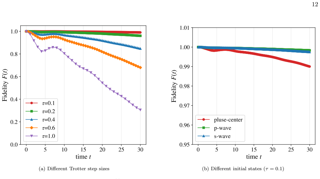
Numerical experiments demonstrate agreement between the quantum-circuit output and exact time evolution while recovering the physical wave fields.

Where Pith is reading between the lines

These are editorial extensions of the paper, not claims the author makes directly.

The same register-separation approach could be extended to media whose material properties vary in space by allowing the Hamiltonian coefficients to become position-dependent operators.
The explicit circuit could be combined with quantum linear-system or optimization routines to solve inverse problems that recover material parameters from observed wave data.
Analogous tensor-product decompositions may simplify Hamiltonian simulation of other first-order vector wave systems in acoustics or electromagnetism.

Load-bearing premise

The finite-difference discretization of the velocity-stress system can be rewritten exactly as a Schrödinger Hamiltonian whose tensor-product structure supports direct and efficient gate decomposition without hidden costs that grow with dimension or material variation.

What would settle it

Execute the circuit for a point-source excitation in uniform material, reconstruct the velocity and stress fields, and test whether the deviation from the known analytic solution stays inside the error bound derived from the Trotter analysis.

Figures

Figures reproduced from arXiv: 2604.20284 by Hiroshi Yano, Kosuke Nakanishi, Yuki Sato.

**Figure 2.** Figure 2: FIG. 2. Fidelity [PITH_FULL_IMAGE:figures/full_fig_p012_2.png] view at source ↗

**Figure 3.** Figure 3: FIG. 3. Comparison of the reconstructed fields [PITH_FULL_IMAGE:figures/full_fig_p013_3.png] view at source ↗

read the original abstract

We present an explicit quantum circuit construction for Hamiltonian simulation of a first-order velocity--stress formulation of the three-dimensional elastic wave equation in homogeneous isotropic media. Previous studies have shown how elastic wave equations can be cast into forms amenable to Hamiltonian simulation, but they typically rely on black box Hamiltonian access assumptions, making gate complexity estimation difficult. Starting from the first-order velocity--stress formulation, we discretize the system by finite differences, transform it into Schr\"odinger form, and exploit the separation between the component register and the spatial register to decompose the Hamiltonian into structured tensor product terms. This yields explicit implementations of first-order and second-order Trotter formulas for the resulting time evolution operator. We derive corresponding error bounds and constant sensitive qubit and CNOT complexity estimates in terms of the discretization parameter, simulation time, target accuracy, and material parameters. Numerical experiments validate the proposed framework through comparisons with the exact time evolution and reconstructed physical fields.

Editorial analysis

A structured set of objections, weighed in public.

Desk editor's note, referee report, simulated authors' rebuttal, and a circularity audit. Tearing a paper down is the easy half of reading it; the pith above is the substance, this is the friction.

Desk Editor's Note private letter to a colleague

The paper offers explicit Trotter circuits and resource estimates for 3D elastic waves but the 3D spatial operator costs need close checking.

read the letter

This paper gives a concrete quantum circuit for simulating the 3D elastic wave equation using Hamiltonian simulation techniques. The authors move past the usual black-box Hamiltonian assumption by providing an explicit decomposition and resource estimates that hardware teams could actually use. They begin with the velocity-stress formulation of the elastic equations in homogeneous isotropic media. After finite-difference discretization on a 3D grid, they recast the system as a Schrödinger Hamiltonian. The key step is separating the small component register (for the nine velocity and stress components) from the spatial register (encoding the grid points). This separation lets them express the Hamiltonian as a sum of tensor-product terms, each involving a component operator and a spatial derivative operator. From there they construct explicit first-order and second-order Trotter circuits, derive error bounds that depend on the discretization parameter, simulation time, target accuracy, and material parameters, and count the qubits and CNOT gates accordingly. Numerical experiments then compare the simulated evolution to the exact solution and reconstruct the physical fields to check consistency. What stands out as new is the explicit gate-level construction for this particular PDE in three dimensions, along with the constant-sensitive complexity formulas. Earlier papers apparently stopped at oracle access, so this fills a practical gap for estimating real costs. The work does well in keeping everything parameter-dependent and in including numerical validation that shows the method recovers the expected wave behavior. The main soft spot is around the implementation of the spatial operators in 3D. Realizing finite-difference stencils or shifts for partial derivatives in x, y, and z on a 3D grid register can require multi-controlled gates or QFT-based methods whose depth might introduce factors that grow with log of the grid size or with the three directions. The paper claims the tensor-product structure keeps everything efficient with constants that do not hide such overheads, but without the detailed circuit diagrams or gate-count breakdowns it is difficult to confirm that no extra scaling sneaks in. If those costs are truly bounded as stated, the estimates hold; otherwise they would need adjustment. The numerical part is reassuring but does not directly test the gate complexity. This is for quantum algorithm researchers focused on classical wave and PDE simulation, and for experimental groups that need ballpark resource numbers. A reader looking for implementable algorithms rather than high-level existence results will get direct value. The paper is coherent and the claims are testable, so it deserves a serious referee who can check the derivations and the 3D circuit details. I would recommend sending it to peer review. The explicitness is a genuine advance worth the effort to verify.

Referee Report

2 major / 2 minor

Summary. The manuscript claims an explicit quantum circuit construction for Hamiltonian simulation of a first-order velocity-stress formulation of the three-dimensional elastic wave equation in homogeneous isotropic media. It discretizes the system via finite differences, transforms it into Schrödinger form, exploits the separation between a component register and a spatial register to decompose the Hamiltonian into structured tensor-product terms, provides explicit first- and second-order Trotter implementations, derives corresponding error bounds together with constant-sensitive qubit and CNOT complexity estimates (in terms of discretization parameter, simulation time, target accuracy, and material parameters), and validates the framework numerically against exact time evolution with reconstruction of physical fields.

Significance. If the central decomposition and explicit gate implementations hold without hidden overheads, the work supplies a concrete, non-black-box resource estimate for quantum simulation of 3D elastic waves. This moves beyond prior abstract Hamiltonian-access assumptions and could support applications in seismic modeling or materials science where quantifiable gate counts are required.

major comments (2)

[Hamiltonian decomposition and circuit construction] The transformation of the finite-difference velocity-stress system into Schrödinger form (described after the discretization step) must be shown to produce an operator that is exactly a sum of terms of the form α_{c,d} (C_c ⊗ D_d), with C_c acting only on the small component register and D_d being purely spatial finite-difference operators on the 3D grid register. Any residual cross-component or cross-direction couplings would prevent the claimed tensor-product decomposition and invalidate the subsequent Trotter circuit constructions and complexity formulas.
[Complexity estimates and error bounds] The constant-sensitive CNOT complexity estimates (given in the complexity analysis section) do not yet explicitly account for the cost of realizing the 3D spatial derivative operators (partial_x, partial_y, partial_z) on the grid register. Standard implementations via QFT-based shifts or direct stencil circuits introduce factors of log N (where N is the discretization parameter) or additional factors of 3 for the three spatial directions; these must be shown to be either absorbed into the stated constants or included in the bounds, as they are load-bearing for the claimed explicit implementations.

minor comments (2)

[Numerical validation] The numerical experiments section should report the specific grid sizes, time-step values, and quantitative error metrics (e.g., L2 norms) used in the comparisons with exact evolution to facilitate reproducibility.
[Preliminaries] Notation for the component register versus the spatial register should be introduced with a clear table or diagram early in the manuscript to avoid ambiguity when discussing tensor-product structure.

Simulated Author's Rebuttal

2 responses · 0 unresolved

We thank the referee for the careful reading and constructive comments. We address the two major comments point by point below, providing clarifications and indicating revisions where appropriate. We believe these responses strengthen the presentation of the explicit circuit constructions and complexity estimates.

read point-by-point responses

Referee: The transformation of the finite-difference velocity-stress system into Schrödinger form (described after the discretization step) must be shown to produce an operator that is exactly a sum of terms of the form α_{c,d} (C_c ⊗ D_d), with C_c acting only on the small component register and D_d being purely spatial finite-difference operators on the 3D grid register. Any residual cross-component or cross-direction couplings would prevent the claimed tensor-product decomposition and invalidate the subsequent Trotter circuit constructions and complexity formulas.

Authors: We thank the referee for this observation. Section III of the manuscript derives the Schrödinger-form Hamiltonian from the discretized first-order velocity-stress system. Under the homogeneous isotropic assumption, the resulting operator is exactly a sum of terms α_{c,d} (C_c ⊗ D_d), where the component operators C_c act only on the 6-dimensional register (three velocity and three stress components) and the D_d are purely spatial finite-difference operators (no cross-direction couplings appear because the material parameters are scalars). The explicit expansion of all 18 terms (accounting for the three spatial directions and the six components) is already present in the derivation, confirming the absence of residual cross terms. To make this structure fully transparent, we will add a dedicated paragraph and table in the revised manuscript that lists every term in the sum and verifies the tensor-product form before proceeding to the Trotter decompositions. revision: yes
Referee: The constant-sensitive CNOT complexity estimates (given in the complexity analysis section) do not yet explicitly account for the cost of realizing the 3D spatial derivative operators (partial_x, partial_y, partial_z) on the grid register. Standard implementations via QFT-based shifts or direct stencil circuits introduce factors of log N (where N is the discretization parameter) or additional factors of 3 for the three spatial directions; these must be shown to be either absorbed into the stated constants or included in the bounds, as they are load-bearing for the claimed explicit implementations.

Authors: We appreciate the referee highlighting the need for explicit accounting of derivative costs. Our complexity formulas are stated as constant-sensitive (rather than purely asymptotic) precisely so that implementation overheads for the spatial operators can be folded into the constants. In the revised manuscript we will insert a short subsection that (i) specifies the chosen implementation of each partial derivative (QFT-based shift with cost O(log N) per direction), (ii) shows that the factor of 3 arising from the three spatial directions is absorbed into the overall constant multiplying the leading term, and (iii) confirms that the log N factor likewise resides inside the stated constants. Because the paper already supplies constant-sensitive rather than leading-order-only bounds, the numerical values of the constants will be updated to reflect these contributions, but the functional dependence on grid size, time, accuracy, and material parameters remains unchanged. revision: partial

Circularity Check

0 steps flagged

No circularity: derivation proceeds from standard first-order equations via explicit discretization and tensor-product decomposition.

full rationale

The paper begins from the established first-order velocity-stress formulation of the 3D elastic wave equation in homogeneous isotropic media, applies standard finite-difference discretization to obtain a discrete operator, recasts it into Schrödinger form by separating the small component register from the spatial grid register, and decomposes the resulting Hamiltonian into explicit tensor-product terms. From this structure it constructs first- and second-order Trotter circuits, derives error bounds via standard Trotter analysis, and obtains qubit/CNOT counts whose leading terms are expressed in terms of the discretization parameter, time, accuracy, and material constants. None of these steps reduces to a self-definition, a fitted parameter renamed as a prediction, or a load-bearing self-citation; the tensor-product decomposition follows directly from the finite-difference stencil on the 9-component system and the product structure of the 3D grid. The construction is therefore self-contained against external benchmarks and receives the default non-circularity finding.

Axiom & Free-Parameter Ledger

0 free parameters · 2 axioms · 0 invented entities

The approach rests on standard numerical-analysis assumptions about finite-difference consistency and on the algebraic fact that the discretized operator can be written as a sum of tensor-product terms; no new physical entities or fitted constants are introduced in the abstract.

axioms (2)

domain assumption Finite-difference discretization of the first-order velocity-stress system yields a Hamiltonian whose spectrum and time evolution remain faithful to the continuous PDE for the chosen grid sizes.
Invoked when the continuous equations are replaced by the discrete matrix.
domain assumption The component and spatial degrees of freedom can be separated into distinct registers so that the Hamiltonian decomposes into a sum of tensor-product operators implementable by elementary gates.
Central to obtaining explicit rather than black-box circuits.

pith-pipeline@v0.9.0 · 5466 in / 1635 out tokens · 32527 ms · 2026-05-10T00:41:41.868951+00:00 · methodology

discussion (0)

Reference graph

Works this paper leans on

38 extracted references · 6 canonical work pages · 1 internal anchor

[1]

H (α) jk , 15X l=1 nX m=1 H (α) lm + nX m=k+1 H (α) jm # , (79) Ξcross αβ := 15X j=0 nX k=1

The first order Trotter formula We analyze the first-order formula: one step error bound, one step implementation cost, and the resulting global complexity. We start from the standard commu- tator scaling bound [30]. Proposition 1(Commutator scaling bound for the first-order Trotter formula: Proposition 9 of Ref. [30]). Let H= RX r=1 Hr,(50) where eachH r...
[2]

(90) The details are given in Appendix B

Hence ∥S−1 comp∥= ( E 1−2ν for 0≤ν < 1 2 , E 1+ν for−1< ν <0. (90) The details are given in Appendix B. Equivalently, we can rewrite ∥S−1 comp∥= max{3K,2µ},(91) where the bulk modulusKand shear modulusµare given by K= E 3(1−2ν) , µ= E 2(1 +ν) .(92) Therefore, the error and gate bound increase with mate- rial stiffness (largeK, µ) and decrease with mass de...
[3]

As in the first-order case, we first state the generic norm scaling error bound, and then specialize it to the Hamiltonian in Eq

The second order Trotter formula We next analyze the second-order formulaU2(τ). As in the first-order case, we first state the generic norm scaling error bound, and then specialize it to the Hamiltonian in Eq. (32) to obtain explicit parameter dependence. Proposition 8(Norm scaling bound for the sec- ond-order Trotter formula: Lemma 1 in Ref. [29]).Let H=...
[4]

pulse” denotes a localized excitation supported on the central 2×2×2 grid block, while “p

Comparison with classical time integration of the same semidiscrete system To make the comparison as direct as possible, we com- pare the quantum algorithm with a classical explicit in- tegrator applied to the same semidiscrete ODE defined by Eq. (25), rather than with a different PDE-level dis- cretization. Since the seven zero-padded components are dyna...
[5]

M. E. Taylor,Partial Differential Equations I: Basic The- ory, Applied Mathematical Sciences, Vol. 115 (Springer International Publishing, Cham, 2023)

2023
[6]

Navier, M´ emoire sur les lois du mouvement des fluides, M´ emoires de l’Acad´ emie des sciences6, 389 (1822)

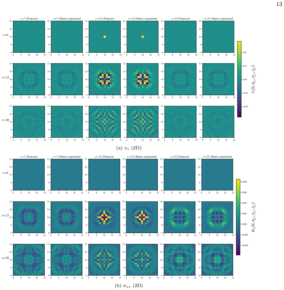
H. Navier, M´ emoire sur les lois du mouvement des fluides, M´ emoires de l’Acad´ emie des sciences6, 389 (1822). 13 0 8 16 24 32 0 8 16 24 32 t = 0 z = 7 | Proposed 0 8 16 24 32 0 8 16 24 32 z = 7 | Matrix exponential 0 8 16 24 32 0 8 16 24 32 z = 15 | Proposed 0 8 16 24 32 0 8 16 24 32 z = 15 | Matrix exponential 0 8 16 24 32 0 8 16 24 32 z = 23 | Propo...
[7]

Aki and P

K. Aki and P. G. Richards,Quantitative Seismology(Uni- versity Science Books, 2002)

2002
[8]

K. J. Marfurt, Accuracy of finite-difference and finite- element modeling of the scalar and elastic wave equa- tions, Geophysics49, 533 (1984)

1984
[9]

R. J. LeVeque, 1. Finite Difference Approximations, in Finite Difference Methods for Ordinary and Partial Dif- ferential Equations(Society for Industrial and Applied Mathematics, 2007) pp. 3–11

2007
[10]

Virieux, H

J. Virieux, H. Calandra, and R.- ´E. Plessix, A review of the spectral, pseudo-spectral, finite-difference and finite- element modelling techniques for geophysical imaging, Geophysical Prospecting59, 794 (2011)

2011
[11]

I. Y. Dodin and E. A. Startsev, On applications of quan- tum computing to plasma simulations, Physics of Plas- mas28, 10.1063/5.0056974 (2021)

work page doi:10.1063/5.0056974 2021
[12]

Krovi, Improved quantum algorithms for linear and nonlinear differential equations, Quantum7, 913 (2023)

H. Krovi, Improved quantum algorithms for linear and nonlinear differential equations, Quantum7, 913 (2023)

2023
[13]

Y. Sato, H. Tezuka, R. Kondo, and N. Yamamoto, Quan- tum algorithm for partial differential equations of non- conservative systems with spatially varying parameters, Phys. Rev. Appl.23, 014063 (2025)

2025
[14]

Meng and Y

Z. Meng and Y. Yang, Quantum computing of fluid dy- namics using the hydrodynamic Schr¨ odinger equation, Phys. Rev. Res.5, 033182 (2023)

2023
[15]

S. Jin, N. Liu, and Y. Yu, Time complexity analysis of quantum algorithms via linear representations for nonlin- 14 ear ordinary and partial differential equations, Journal of Computational Physics487, 112149 (2023)

2023
[16]

A. W. Harrow, A. Hassidim, and S. Lloyd, Quantum Algorithm for Linear Systems of Equations, Phys. Rev. Lett.103, 150502 (2009)

2009
[17]

S. Jin, N. Liu, and Y. Yu, Quantum Simulation of Partial Differential Equations via Schr¨ odingerization, Phys. Rev. Lett.133, 230602 (2024)

2024
[18]

S. Jin, N. Liu, and Y. Yu, Quantum simulation of partial differential equations: Applications and detailed analy- sis, Phys. Rev. A108, 032603 (2023)

2023
[19]

An, J.-P

D. An, J.-P. Liu, and L. Lin, Linear combination of Hamiltonian simulation for nonunitary dynamics with optimal state preparation cost, Phys. Rev. Lett.131, 150603 (2023)

2023
[20]

Y. Sato, R. Kondo, I. Hamamura, T. Onodera, and N. Yamamoto, Hamiltonian simulation for hyperbolic partial differential equations by scalable quantum cir- cuits, Phys. Rev. Res.6, 033246 (2024)

2024
[21]

P. C. S. Costa, S. Jordan, and A. Ostrander, Quantum algorithm for simulating the wave equation, Phys. Rev. A99, 012323 (2019)

2019
[22]

Babbush, D

R. Babbush, D. W. Berry, R. Kothari, R. D. Somma, and N. Wiebe, Exponential Quantum Speedup in Simulating Coupled Classical Oscillators, Phys. Rev. X13, 041041 (2023)

2023
[23]

B¨ osch, M

C. B¨ osch, M. Schade, G. Aloisi, S. D. Keating, and A. Fichtner, Quantum wave simulation with sources and loss functions, Phys. Rev. Res.7, 033225 (2025)

2025
[24]

Schade, C

M. Schade, C. B¨ osch, V. Hapla, and A. Fichtner, A quan- tum computing concept for 1-D elastic wave simulation with exponential speedup, Geophysical Journal Interna- tional238, 321 (2024)

2024
[25]

S. Jin, Z. Tang, X. Yin, and L. Zhang, Quantum Circuits for the Black-Scholes equations via Schr¨ odingerisation (2025), arXiv:2505.04304 [quant-ph]

work page arXiv 2025
[26]

C. Ma, S. Jin, N. Liu, K. Wang, and L. Zhang, Schr¨ odingerization based Quantum Circuits for Maxwell’s Equation with time-dependent source terms (2024), arXiv:2411.10999 [quant-ph]

work page arXiv 2024
[27]

Jin and C

S. Jin and C. Zhang, Quantum simulation of elas- tic wave equations via Schr¨ odingerisation (2025), arXiv:2505.18711 [quant-ph]

work page arXiv 2025
[28]

Kiffner and D

M. Kiffner and D. Jaksch, Tensor network reduced or- der models for wall-bounded flows, Phys. Rev. Fluids8, 124101 (2023)

2023
[29]

G. H. Low and I. L. Chuang, Hamiltonian Simulation by Qubitization, Quantum3, 163 (2019)

2019
[30]

G. H. Low and I. L. Chuang, Optimal Hamiltonian Sim- ulation by Quantum Signal Processing, Phys. Rev. Lett. 118, 010501 (2017)

2017
[31]

Gily´ en, Y

A. Gily´ en, Y. Su, G. H. Low, and N. Wiebe, Quantum singular value transformation and beyond: Exponential improvements for quantum matrix arithmetics, inPro- ceedings of the 51st Annual ACM SIGACT Symposium on Theory of Computing(2019) pp. 193–204

2019
[32]

Lloyd, Universal Quantum Simulators, Science273, 1073 (1996)

S. Lloyd, Universal Quantum Simulators, Science273, 1073 (1996)

1996
[33]

D. W. Berry, G. Ahokas, R. Cleve, and B. C. Sanders, Ef- ficient quantum algorithms for simulating sparse Hamil- tonians, Commun. Math. Phys.270, 359 (2007)

2007
[34]

A. M. Childs, Y. Su, M. C. Tran, N. Wiebe, and S. Zhu, Theory of Trotter Error with Commutator Scaling, Phys. Rev. X11, 011020 (2021)

2021
[35]

R. Vale, T. M. D. Azevedo, I. C. S. Ara´ ujo, I. F. Araujo, and A. J. da Silva, Circuit Decomposition of Multicon- trolled Special Unitary Single-Qubit Gates, IEEE Trans- actions on Computer-Aided Design of Integrated Circuits and Systems43, 802 (2024)

2024
[36]

M. A. Nielsen and I. L. Chuang,Quantum Computation and Quantum Information: 10th Anniversary Edition (Cambridge University Press, Cambridge ; New York, 2010)

2010
[37]

Lecture notes on quantum algorithms for scientific computation.arXiv preprint arXiv:2201.08309, 2022

L. Lin, Lecture Notes on Quantum Algorithms for Scien- tific Computation (2022), arXiv:2201.08309 [quant-ph]

work page arXiv 2022
[38]

Quantum computing with Qiskit

A. Javadi-Abhari, M. Treinish, K. Krsulich, C. J. Wood, J. Lishman, J. Gacon, S. Martiel, P. D. Nation, L. S. Bishop, A. W. Cross, B. R. Johnson, and J. M. Gambetta, Quantum computing with Qiskit (2024), arXiv:2405.08810 [quant-ph]. 15 Appendix A: Auxiliary Lemmas and Deferred Proof for the First-Order Commutator Bound In the following,∥·∥ tr denotes trac...

work page internal anchor Pith review arXiv 2024