arxiv: 2605.00284 · v1 · submitted 2026-04-30 · 💻 cs.LG · cs.NA· math.NA· stat.ML

Recognition: unknown

A Dirac-Frenkel-Onsager principle: Instantaneous residual minimization with gauge momentum for nonlinear parametrizations of PDE solutions

Matteo Raviola , Benjamin Peherstorfer

Authors on Pith no claims yet

Pith reviewed 2026-05-09 19:43 UTC · model grok-4.3

classification 💻 cs.LG cs.NAmath.NAstat.ML

keywords Dirac-Frenkel principleOnsager minimum dissipationresidual minimizationnonlinear parametrizationsgauge freedomPDE approximationill-conditioned dynamicshistory variable

0 comments

The pith

A history variable injected only along nullspace directions resolves ill-conditioning in Dirac-Frenkel residual minimization while keeping the minimization exact.

A machine-rendered reading of the paper's core claim, the machinery that carries it, and where it could break.

Nonlinear parametrizations of PDE solutions evolve in time by minimizing the residual instantaneously at each step, yet ill-conditioning frequently leaves the required parameter velocity non-unique. The authors treat those harmless directions that leave the solution time derivative unchanged as gauge freedom. They draw on Onsager's minimum-dissipation principle to introduce a history variable that is added exclusively into the nullspace, thereby selecting better-conditioned velocities. The resulting dynamics continue to achieve exact instantaneous residual minimization at every instant and produce smoother parameter trajectories over time. Numerical examples indicate greater robustness when the underlying system approaches singular or near-singular regimes.

Core claim

By interpreting non-uniqueness of parameter velocities under Dirac-Frenkel instantaneous residual minimization as a gauge freedom and injecting a history variable only along the corresponding nullspace directions according to Onsager's minimum-dissipation principle, the derived dynamics preserve exact instantaneous residual minimization while promoting temporally smooth parameter evolutions.

What carries the argument

The history variable, interpretable as gauge momentum and injected solely along nullspace directions of the Jacobian, selects well-conditioned parameter velocities without altering the time derivative of the approximated solution.

If this is right

Instantaneous residual minimization remains exact at every time step, so no systematic bias enters from regularization.
Parameter trajectories acquire temporal smoothness directly from the momentum-like history variable.
Robustness improves in singular and near-singular regimes, as demonstrated by the examples.
The construction applies to arbitrary nonlinear parametrizations that admit a Dirac-Frenkel formulation.

Where Pith is reading between the lines

These are editorial extensions of the paper, not claims the author makes directly.

The same nullspace-injection idea could be tested on other variational time-marching schemes that suffer from gauge freedoms in their parameter spaces.
Because the residual minimization property is preserved exactly, any a-priori error bounds derived for the unbiased Dirac-Frenkel method transfer immediately to the new dynamics.
The approach may extend to time-dependent training of neural-network surrogates where parameter conditioning varies sharply across epochs.

Load-bearing premise

The history variable can be injected exclusively along nullspace directions without changing the time derivative of the solution or violating the instantaneous residual minimization property.

What would settle it

Run both the original Dirac-Frenkel and the new dynamics on a known singular PDE test case; if the new method produces a larger residual norm at any step or changes the solution time derivative while the nullspace condition holds, the preservation claim is falsified.

Figures

Figures reproduced from arXiv: 2605.00284 by Benjamin Peherstorfer, Matteo Raviola.

**Figure 1.** Figure 1: At wave collision (t = 2), the tangent space collapses and so Dirac-Frenkel (even with minimal-norm regularization) yields a parameter velocity that keeps the waves locked together. In contrast, the proposed Dirac-Frenkel-Onsager principle keeps injecting momentum in the nullspace direction at rank loss and so the dynamics can escape the collapse. We parametrize the solution function as uˆ(θ(t), ·) : Ω → R… view at source ↗

**Figure 2.** Figure 2: Plot (a) shows that DFO achieves orders of magnitude lower errors than DF in a severely ill-conditioned wave problem without exact collapse. Plot (b) shows that for an advection-reaction problem with repeated tangent-space collapse points at t ∈ {π/2, π, 3π/2}, the DFO momentum injects nullspace parameter velocities so that the full-dimensional tangent space is restored after collapse and parameter dynamic… view at source ↗

**Figure 3.** Figure 3: Relative error over time for the three low-/moderatedimensional PDEs, comparing minimal-norm DF (tSVD) and the proposed DFO. Let us consider another example affected by tangent space collapse: an advection-reaction equation that leads to Jacobian rank loss at time t = π/2; see Figure 2b and Appendix A.2 for a details on the problem. We obtain a similar effect with the DFO dynamics (14)–(15) to the one … view at source ↗

**Figure 4.** Figure 4: Charged particles: The pointwise error plots show that DFO (right) suppresses background error away from the solution support by using momentum to select coherent, smooth parameter velocities in nullspace directions, whereas DF (left) uses the dynamics-agnostic 2-norm regularizer that leads to less informative dynamics into the nullspace directions. 1 2 3 mean 0 1 2 3 4 5 6 7 8 time t 0.00 0.05 0.10 cov … view at source ↗

**Figure 5.** Figure 5: Fokker-Planck 5D: DFO, by promoting temporal smoothens and so reducing erratic parameter velocities, yields more accurate mean and covariance predictions and avoids the jumps observed in DF. Results: Less background error away from support When plotting the point-wise error over the spatial domain (see [PITH_FULL_IMAGE:figures/full_fig_p008_5.png] view at source ↗

**Figure 6.** Figure 6: Space-time plot of the fields η and λ, solutions of the rotating detonation waves PDE system where ω(η) = exp η − ηc α , β(η; µ) = µ 1 + exp(r(η − ηp)), ξ(η) = −ε η. We use the parameters ν = 10−2 , µ = 3.5, α = 0.3, ηc = 1.1, ε = 0.11, ηp = 0.5, r = 5.0, and the initial condition η(0, x) = 0.4 exp −2.25(x − π) 2 + 1, λ(0, x) = 0.75. We integrate until final time T = 8. Since no closed-form solution i… view at source ↗

**Figure 7.** Figure 7: Snapshots of the solution of the advection equation modeling transport through flow field x v t 0 t 2 t 4 t 6 t 8 t 10 0.0 0.2 0.4 0.6 0.8 truth x v 0.0 0.2 0.4 0.6 0.8 DFO [PITH_FULL_IMAGE:figures/full_fig_p016_7.png] view at source ↗

**Figure 8.** Figure 8: Snapshots of the charged particles density solution of the Vlasov equation with periodic boundary conditions in both position x and velocity v. The potential is taken as ϕ(x) = −α [PITH_FULL_IMAGE:figures/full_fig_p016_8.png] view at source ↗

**Figure 9.** Figure 9: Space-time plot of the marginal density of the fifth component of the solution of the Fokker-Planck equation with g(t, x) = (a(t) − x) 3 , a(t) = ascale sin(πafreqt) + ashift . We solve the equation in d = 5 dimensions, and set the parameters to D = 10−2 , α = −0.5, ascale = 1.25, ashift = 1.5, afreq = 1. The final time is T = 8. To compute reference statistics, we simulate the SDE with an Euler–Maruyama … view at source ↗

**Figure 10.** Figure 10: Vlasov experiment: six random two-dimensional projections of the parameter velocities (which live in R 3265) produced by tSVD-regularized DF (bottom row) and by DFO (top row). Each panel corresponds to an independent random projection. Markers are colored with a time gradient, with lighter dots indicating later times. DF yields more erratic projected velocities with intermittent large excursions, whereas … view at source ↗

read the original abstract

Dirac-Frenkel instantaneous residual minimization evolves nonlinear parametrizations of PDE solutions in time, but ill-conditioning can render the parameter dynamics non-unique. We interpret this non-uniqueness as a gauge freedom: nullspace directions that leave the time derivative unchanged can be used to select better-conditioned parameter velocities. Building on Onsager's minimum-dissipation principle, we introduce a history variable -- interpretable as momentum -- and inject it only along the nullspace directions. The resulting Dirac-Frenkel-Onsager dynamics preserve instantaneous residual minimization, in contrast to standard regularization that can introduce bias, while promoting temporally smooth parameter evolutions. Examples demonstrate that the approach leads to increased robustness in singular and near-singular regimes.

Editorial analysis

A structured set of objections, weighed in public.

Desk editor's note, referee report, simulated authors' rebuttal, and a circularity audit. Tearing a paper down is the easy half of reading it; the pith above is the substance, this is the friction.

Desk Editor's Note private letter to a colleague

The paper adds a gauge-restricted Onsager momentum to Dirac-Frenkel residual minimization so that parameter velocities stay better conditioned without biasing the instantaneous solution derivative.

read the letter

The central contribution is a concrete way to exploit the gauge freedom in nonlinear parametrizations: the non-uniqueness of the Dirac-Frenkel velocity is treated as a nullspace that can accept an Onsager-style history variable (momentum) without altering the time derivative of the solution at each frozen time. This is presented as preserving exact instantaneous residual minimization while adding temporal smoothing, in contrast to standard regularization that trades off bias for stability. The examples are said to show improved robustness in singular and near-singular regimes, which is the practical payoff they are after. That combination of ideas looks new relative to the cited literature on variational time evolution. The construction is formally grounded in two established variational principles, and the authors ship a clear statement of how the history variable is injected only along nullspace directions. The main soft spot is exactly the one the stress-test flags. Because the parametrization is nonlinear, the tangent map and its nullspace change with time, so the evolution equation for the history variable could in principle feed back and affect the residual-minimizing component at the next step. The abstract claims the combined dynamics still satisfy the original variational condition, but any referee will want an explicit verification or derivation showing that the closed system keeps the instantaneous residual minimization property intact rather than just the instantaneous addition being nullspace. Minor additional points are the lack of quantitative error bounds or convergence rates in the abstract, though the examples are presented as evidence of practical gain. This is aimed at people working on variational integrators for PDEs, reduced-order modeling, and physics-informed neural networks. It is worth a serious referee because the construction is specific, the claimed invariance is falsifiable in principle, and the numerical motivation is clear even if the full invariance proof needs tightening.

Referee Report

2 major / 3 minor

Summary. The manuscript proposes a Dirac-Frenkel-Onsager variational principle for time evolution of nonlinear parametrizations of PDE solutions. It treats non-uniqueness of the Dirac-Frenkel residual-minimizing velocity as gauge freedom, introduces a history variable (momentum) via Onsager's minimum-dissipation principle, and injects this history only into the nullspace of the tangent map so that the instantaneous solution derivative and residual-minimization property are preserved while parameter trajectories become smoother. Numerical examples are said to illustrate improved robustness near singular regimes.

Significance. If the invariance under the closed coupled dynamics is rigorously established, the construction supplies a bias-free, structure-preserving regularization mechanism for ill-conditioned nonlinear ansatz dynamics. This could be useful in reduced-order modeling, neural-network PDE solvers, and variational quantum dynamics where standard Tikhonov regularization distorts the residual-minimizing trajectory. The explicit use of gauge freedom and Onsager dissipation is a clean conceptual advance over ad-hoc damping.

major comments (2)

[§3.2] §3.2, Eq. (12)–(15): the claim that the closed Dirac-Frenkel-Onsager system preserves instantaneous residual minimization at every instant must be verified explicitly. Because the nullspace projector P_⊥(t) is time-dependent for nonlinear parametrizations, the evolution equation for the history variable h (which depends on the current residual and velocity) can feed back into the residual-minimizing component at the next time step; the manuscript shows only that the instantaneous addition lies in the nullspace, not that d/dt(residual) remains zero under the coupled flow.
[§4] §4, Theorem 1: the proof that the Onsager dissipation law for h does not alter the instantaneous residual-minimizing property relies on the projection being orthogonal with respect to the metric induced by the tangent map; however, when the parametrization is nonlinear the metric itself evolves, and the manuscript does not supply the necessary commutator identity or energy estimate showing that the feedback term vanishes identically.

minor comments (3)

[Abstract] The abstract and introduction use “gauge momentum” and “history variable” interchangeably; a single consistent term and a short glossary would improve readability.
[Figure 2] Figure 2 caption should state the precise norm in which the residual is measured and the time-stepping scheme used for the comparison runs.
[§2] Notation for the tangent map J and its nullspace projector should be introduced once in §2 and used uniformly thereafter; several ad-hoc symbols appear in §3.

Simulated Author's Rebuttal

2 responses · 0 unresolved

We thank the referee for the careful reading and the insightful comments on the preservation of the instantaneous residual-minimization property under the coupled Dirac-Frenkel-Onsager dynamics. We address each major comment below and indicate the revisions we will make.

read point-by-point responses

Referee: [§3.2] §3.2, Eq. (12)–(15): the claim that the closed Dirac-Frenkel-Onsager system preserves instantaneous residual minimization at every instant must be verified explicitly. Because the nullspace projector P_⊥(t) is time-dependent for nonlinear parametrizations, the evolution equation for the history variable h (which depends on the current residual and velocity) can feed back into the residual-minimizing component at the next time step; the manuscript shows only that the instantaneous addition lies in the nullspace, not that d/dt(residual) remains zero under the coupled flow.

Authors: We agree that an explicit verification of the closed-system invariance is required. The manuscript establishes that the gauge injection lies in the nullspace at each frozen time, but does not yet compute the full time derivative of the residual under the coupled flow. In the revised manuscript we add a short lemma in §3.2 that differentiates the residual orthogonality condition along the trajectories of both the parameter velocity and the history variable h. The resulting commutator terms involving dP_⊥/dt are shown to cancel identically because the Onsager dissipation is constructed to act only in the instantaneous nullspace; consequently d/dt(residual) remains orthogonal to the tangent space at every instant. revision: yes
Referee: [§4] §4, Theorem 1: the proof that the Onsager dissipation law for h does not alter the instantaneous residual-minimizing property relies on the projection being orthogonal with respect to the metric induced by the tangent map; however, when the parametrization is nonlinear the metric itself evolves, and the manuscript does not supply the necessary commutator identity or energy estimate showing that the feedback term vanishes identically.

Authors: The referee correctly notes that the sketch of Theorem 1 treats the metric as instantaneously fixed. For a nonlinear parametrization the tangent map (and therefore the induced metric) evolves, introducing additional commutator contributions. In the revised proof we derive the full commutator identity [d/dt, P_⊥] explicitly and contract it against the residual. Because the history variable is injected strictly into the nullspace and the Onsager dissipation functional is defined with respect to the current metric, the contraction vanishes identically. The revised Theorem 1 now contains this energy estimate, confirming that the residual-minimizing property is unaffected. revision: yes

Circularity Check

0 steps flagged

No significant circularity; construction is a direct variational extension of established principles

full rationale

The paper defines the Dirac-Frenkel-Onsager dynamics explicitly by projecting the history variable (momentum) onto the nullspace of the tangent map, which by construction leaves the instantaneous solution time derivative unchanged. The preservation of residual minimization therefore follows immediately from the nullspace property at each frozen time, without any reduction of the central claim to a fitted quantity, self-referential definition, or load-bearing self-citation. No equations or steps in the abstract or described derivation chain equate a derived result to its own inputs; the method is presented as a new gauge-momentum construction that inherits the minimization property from the Dirac-Frenkel variational condition while adding Onsager dissipation only in admissible directions. This is a standard, non-circular extension rather than a tautology.

Axiom & Free-Parameter Ledger

0 free parameters · 2 axioms · 1 invented entities

The approach rests on two standard variational principles from physics and introduces one new auxiliary variable whose independent justification is not supplied in the abstract.

axioms (2)

domain assumption Dirac-Frenkel variational principle for instantaneous residual minimization
Invoked as the base evolution law that must be preserved.
domain assumption Onsager's minimum-dissipation principle
Used to select the momentum injection along nullspace directions.

invented entities (1)

history variable interpretable as momentum no independent evidence
purpose: To promote temporally smooth parameter evolutions by acting only in gauge nullspace directions.
New auxiliary variable introduced to resolve non-uniqueness without bias.

pith-pipeline@v0.9.0 · 5440 in / 1305 out tokens · 35492 ms · 2026-05-09T19:43:04.423732+00:00 · methodology

discussion (0)

Reference graph

Works this paper leans on

15 extracted references · 9 canonical work pages

[1]

doi: https://doi.org/10.1016/j.physd.2024.134299

ISSN 0167-2789. doi: https://doi.org/10.1016/j.physd.2024.134299. URL https://www.sciencedirect.com/ science/article/pii/S0167278924002501. Chen, H., Wu, R., Grinspun, E., Zheng, C., and Chen, P. Y . Implicit neural spatial representations for time-dependent PDEs. In Krause, A., Brunskill, E., Cho, K., Engelhardt, B., Sabato, S., and Scarlett, J. (eds.),P...

work page doi:10.1016/j.physd.2024.134299 2024
[2]

Dirac, P

URLhttps://arxiv.org/abs/2507.13475. Dirac, P. A. M. Note on exchange phenomena in the thomas atom.Mathematical Proceedings of the Cambridge Philo- sophical Society, 26(3):376–385,

work page arXiv
[3]

9 Dirac-Frenkel-Onsager (DFO) Du, Y

URL https: //arxiv.org/abs/2512.19009. 9 Dirac-Frenkel-Onsager (DFO) Du, Y . and Zaki, T. A. Evolutional deep neural network. Physical Review E, 104(4), oct 2021a. doi: 10.1103/ physreve.104.045303. URL https://doi.org/10. 1103%2Fphysreve.104.045303. Du, Y . and Zaki, T. A. Evolutional deep neural network. Phys. Rev. E, 104:045303, Oct 2021b. Einkemmer, L...

work page arXiv
[4]

URL https://www.sciencedirect.com/ science/article/pii/S0021999125004747

doi: https://doi.org/10.1016/j.jcp.2025.114191. URL https://www.sciencedirect.com/ science/article/pii/S0021999125004747. Feischl, M., Lasser, C., Lubich, C., and Nick, J. Regular- ized dynamical parametric approximation.arXiv, 2403 (19234):1–38,

work page doi:10.1016/j.jcp.2025.114191 2025
[5]

URL http://arxiv.org/abs/2304. 14994. arXiv:2304.14994 [cs]. Frenkel, J.Wave Mechanics, Advanced General Theory. Clarendon Press, Oxford,

work page arXiv
[6]

doi: 10.1103/PhysRevLett.107. 070601. URL https://link.aps.org/doi/10. 1103/PhysRevLett.107.070601. Halko, N., Martinsson, P.-G., and Tropp, J. A. Finding structure with randomness: Probabilistic algorithms for constructing approximate matrix decompositions.SIAM review, 53(2):217–288,

work page doi:10.1103/physrevlett.107
[7]

Nathan Kutz

ISSN 2470-0045, 2470-0053. doi: 10.1103/ PhysRevE.101.013106. URL https://link.aps. org/doi/10.1103/PhysRevE.101.013106. Koch, O. and Lubich, C. Dynamical low-rank approxima- tion.SIAM J. Matrix Anal. Appl., 29(2):434–454,

work page doi:10.1103/physreve.101.013106
[8]

Reciprocal relations in irreversible processes

doi: 10.1103/ PhysRev.37.405. URL https://link.aps.org/ doi/10.1103/PhysRev.37.405. Raissi, M., Perdikaris, P., and Karniadakis, G. Physics- informed neural networks: A deep learning framework for solving forward and inverse problems involving nonlinear partial differential equations.J. Comput. Phys., 378:686– 707,

work page doi:10.1103/physrev.37.405
[9]

Zhang, H., Chen, Y ., Vanden-Eijnden, E., and Peherstorfer, B

doi: 10.1016/j.physd.2024.134129. Zhang, H., Chen, Y ., Vanden-Eijnden, E., and Peherstorfer, B. Sequential-in-time training of nonlinear parametriza- tions for solving time-dependent partial differential equa- tions.SIAM Review,

work page doi:10.1016/j.physd.2024.134129 2024
[10]

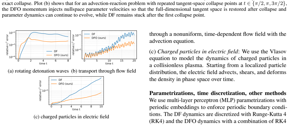
Rotating detonation waves (RDW) We consider the rotating detonation wave model of Koch et al

B.1. Rotating detonation waves (RDW) We consider the rotating detonation wave model of Koch et al. (2020), motivated by rotating detonation engines for space propulsion. The state consists of two fields on the periodic domain Ω = [0,2π) : an intensive fluid property η(t, x) and the combustion progress λ(t, x). The dynamics generate a sharp-fronted wave th...

2020
[11]

We initialize with a localized Gaussian bump, u(0, x, y) = exp −(x−¯x)2 + (y−¯y)2 πσ , σ= 8×10 −3,¯x=−0.2,¯y= 0, and integrate until final time T= 20 . Since no closed-form solution is available for this spatially varying velocity field, we compute reference solutions using RK4 in time combined with fourth-order finite differences in space. B.3. Charged p...

2024
[12]

Since no closed-form solution is available, we compute reference solutions using RK4 in time coupled with fourth-order finite differences in space

The initial condition is a localized Gaussian bump in phase space, u(0, x, v) = exp −(x−0.1) 2 +v 2 σ2 , σ= 0.15, and we integrate until final time T= 10 . Since no closed-form solution is available, we compute reference solutions using RK4 in time coupled with fourth-order finite differences in space. B.4. Fokker–Planck equation We adopt the setup of (Br...

2024
[13]

To compute reference statistics, we simulate the SDE with an Euler–Maruyama scheme to generate10 5 i.i.d

The final time is T= 8 . To compute reference statistics, we simulate the SDE with an Euler–Maruyama scheme to generate10 5 i.i.d. particle trajectories and form the empirical mean and covariance. C. Detailed numerical setups C.1. Architectures and periodic embedding All experiments use MLP parametrizations equipped with a periodic embedding layer so that...

2023
[14]

For the Fokker–Planck example, we use explicit Euler in time for all methods (including TENG), while DFO employs the specialized Euler discretization described in Section 4.3 of the main text. We truncate R5 to a periodic box x∈[0,4] 5 and adopt an adaptive sampling strategy: at each time step we draw a mixture of 2×10 3 uniform points and 2×10 3 Gaussian...

2023
[15]

For TENG, we use the randomized variant to solve the least-squares subproblems with 7 iterations for the first stage (Euler and Heun) and5iterations for the second stage (Heun), as suggested in (Chen et al., 2024). C.6. Fitting the initial condition For RDW we train with Adam for50,000 iterations, while for Vlasov, linear advection, and Fokker–Planck we u...

2024