arxiv: 2605.02274 · v1 · submitted 2026-05-04 · 📊 stat.ME

Recognition: 3 theorem links

· Lean Theorem

Practical Boundary Degeneracy and Reverse-Martingale Limits in Sequential Binary Models

Yuan-chin Ivan Chang

Authors on Pith no claims yet

Pith reviewed 2026-05-08 19:22 UTC · model grok-4.3

classification 📊 stat.ME

keywords boundary degeneracyreverse martingalesequential binary modelsstopping ruleslogistic regression separationBernoulli trialstrajectory stability

0 comments

The pith

Finite sequential binary data justify practical statements like p at most epsilon but never exact boundary values of zero or one.

A machine-rendered reading of the paper's core claim, the machinery that carries it, and where it could break.

The paper argues that runs of all failures or successes in Bernoulli trials, complete separation in logistic regression, and controlled risk paths all reflect the same underlying structure in sequential data. Finite observations allow confident claims that a probability lies at or below a small positive number epsilon or at or above one minus epsilon, yet they never justify declaring the probability exactly zero or one. A reverse-martingale framework unifies these cases and produces a stopping rule that checks three things at once: how close the current estimate sits to the boundary, how wide the uncertainty interval remains, and whether the trajectory has stabilized. This recasts apparent degeneracy as a feature of the limiting conditional expectation rather than a finite-sample certainty. Numerical checks across the three settings show that boundary closeness by itself often misleads while the added stability condition distinguishes lasting limits from temporary appearances.

Core claim

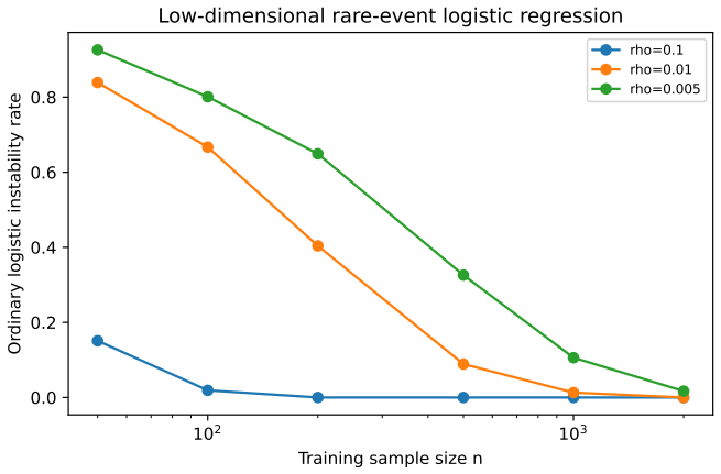
Boundary degeneracy in sequential binary models is a property of the limiting conditional law M_infinity equals the conditional expectation of Y given the sigma-field at infinity, not an exact finite-sample event. This leads to a stopping time tau_RM that simultaneously requires boundary closeness B_n less than or equal to epsilon, uncertainty width W_n less than or equal to w, and trajectory stability r_n less than or equal to eta. The same framework covers Bernoulli rare-event sequences, low- and high-dimensional logistic regression with complete separation, and controlled risk trajectories, showing that boundary closeness alone supplies an unreliable stopping signal.

What carries the argument

The reverse-martingale limit M_infinity equals E(Y given G_infinity) together with the three-condition stopping rule tau_RM that enforces boundary closeness, uncertainty width, and trajectory stability simultaneously.

If this is right

Analysts should replace simple boundary checks with the three-condition stopping rule when declaring practical limits on probabilities.
In rare-event Bernoulli sequences, claims of the form p less than or equal to epsilon become reliable only after trajectory stability is verified.
Complete separation in logistic regression indicates limiting degeneracy only when the added stability condition holds.
The reverse-martingale approach complements classical one-sided binomial tests and sequential probability ratio tests rather than replacing them.
Numerical studies confirm that the stability condition separates transient apparent certainty from genuine limiting degeneracy across the examined settings.

Where Pith is reading between the lines

These are editorial extensions of the paper, not claims the author makes directly.

The same stability requirement could be tested in sequential models with continuous rather than binary outcomes.
Many published reports of exact zero probabilities in empirical sequential studies may be overstated when stability was not checked.
The reverse-martingale perspective may link to broader martingale convergence results used in other areas of sequential analysis.

Load-bearing premise

The reverse-martingale structure and the three stopping conditions apply uniformly to Bernoulli rare-event trials, logistic regression complete separation, and controlled risk trajectories.

What would settle it

A concrete data set or simulation in which the three conditions of tau_RM are all satisfied yet the long-run frequency remains bounded away from the claimed boundary would show that the stability requirement is unnecessary.

Figures

Figures reproduced from arXiv: 2605.02274 by Yuan-chin Ivan Chang.

**Figure 1.** Figure 1: Exact probability of an apparent zero Bernoulli MLE, view at source ↗

**Figure 2.** Figure 2: Instability rate of ordinary logistic regression in the low-dimensional rare-event experi view at source ↗

**Figure 3.** Figure 3: Ordinary logistic instability in the high-dimensional rare-event experiment. Instability view at source ↗

**Figure 4.** Figure 4: Mean simulated conditional-risk trajectories in the reverse-martingale-style stability ex view at source ↗

**Figure 5.** Figure 5: Instability rate in the RAND HIE poor-health rare-event illustration. The outcome view at source ↗

read the original abstract

A run of all failures, a run of all successes, or complete separation in a logistic regression each tempts the analyst to declare a probability of exactly zero or one. The central message of this paper is that all three phenomena share a common structure: finite sequential data justify practical boundary statements of the form $p\leq\varepsilon$ or $p\geq1-\varepsilon$, but not exact boundary probabilities. The paper's contribution is to unify these three settings under a single reverse-martingale framework and to derive a stopping rule, $\tau_{\mathrm{RM}}$, that requires three conditions simultaneously -- boundary closeness $B_n\leq\varepsilon$, uncertainty width $W_n\leq w$, and trajectory stability $r_n\leq\eta$ -- rather than boundary closeness alone. The reverse-martingale view recasts boundary degeneracy as a property of the limiting conditional law $M_\infty=\E(Y\given\G_\infty)$ rather than a finite-sample event, complementing classical one-sided binomial tests and Wald's sequential probability ratio test without replacing them. Numerical studies across Bernoulli rare-event trials, low- and high-dimensional logistic regression, controlled risk trajectories, and a real health-economics data set demonstrate that boundary closeness alone is an unreliable stopping signal, and that the stability condition separates transient apparent certainty from genuine limiting degeneracy.

Editorial analysis

A structured set of objections, weighed in public.

Desk editor's note, referee report, simulated authors' rebuttal, and a circularity audit. Tearing a paper down is the easy half of reading it; the pith above is the substance, this is the friction.

Desk Editor's Note private letter to a colleague

The paper unifies runs of successes/failures and logistic separation under reverse-martingales, showing that a three-condition stopping rule is more reliable than boundary closeness alone.

read the letter

The main takeaway is that finite sequential binary data support practical statements like p ≤ ε but not exact boundary probabilities, and the paper unifies three settings—runs of failures, runs of successes, and logistic complete separation—under a reverse-martingale limit M_∞ = E[Y | G_∞]. It derives a stopping rule τ_RM that waits simultaneously for boundary closeness B_n ≤ ε, uncertainty width W_n ≤ w, and trajectory stability r_n ≤ η, rather than stopping on closeness by itself. This complements classical binomial tests and SPRT without replacing them. The numerical studies across Bernoulli rare-event trials, low- and high-dimensional logistic regression, controlled risk trajectories, and a health-economics dataset illustrate that boundary closeness alone can be unreliable while the stability condition helps separate transient appearances from genuine limiting degeneracy. That empirical check is useful and directly addresses the practical temptation to declare p=0 or 1 too early. The reverse-martingale recasting is a clean conceptual move that avoids reducing the problem to fitted parameters from the same data. On the soft spots, the abstract leaves the exact steps deriving τ_RM from M_∞ and the precise definition of the stability metric r_n somewhat implicit, so the full paper needs to lay those out clearly to confirm uniform applicability without hidden assumptions on the filtration or the metric. The real-data example adds relevance, but sensitivity to parameter choices in the simulations would strengthen the case. This is for statisticians working on sequential monitoring, rare-event detection, or regression with separation risks. A reader focused on practical stopping rules in binary data will find the framework and the evidence that one condition is insufficient worth their time. I would send it to peer review; the core argument is internally consistent, grounded in standard martingale theory, and backed by targeted numerics that make the contribution concrete.

Referee Report

2 major / 2 minor

Summary. The paper claims that phenomena such as runs of all failures or successes in Bernoulli trials and complete separation in logistic regression share a common structure under a reverse-martingale framework. Finite sequential data justify practical boundary statements of the form p ≤ ε or p ≥ 1-ε but not exact boundary probabilities. The contribution is to unify these settings and derive a stopping rule τ_RM requiring simultaneous boundary closeness B_n ≤ ε, uncertainty width W_n ≤ w, and trajectory stability r_n ≤ η, rather than boundary closeness alone. This recasts degeneracy as a property of the limiting conditional law M_∞ = E[Y | G_∞] and is supported by numerical studies across Bernoulli rare-event trials, low- and high-dimensional logistic regression, controlled risk trajectories, and a health-economics dataset showing that boundary closeness alone is unreliable.

Significance. If the results hold, the work provides a unified reverse-martingale approach to practical boundary inference in sequential binary models, complementing but not replacing classical one-sided binomial tests and Wald's SPRT. The three-condition stopping rule and the demonstration that stability separates transient from genuine degeneracy across diverse settings could improve reliability in applications involving rare events or separation, with the numerical studies adding empirical support.

major comments (2)

[Derivation of τ_RM and M_∞] The central unification relies on the reverse-martingale limit M_∞ and the derivation of τ_RM from it; the manuscript should expand the explicit steps connecting the three simultaneous conditions (B_n, W_n, r_n) to this limit, particularly showing uniform applicability to the logistic regression complete-separation case without additional assumptions on the filtration G_∞.
[Numerical studies] The numerical studies are described as demonstrating that the stability condition r_n ≤ η separates transient apparent certainty from genuine limiting degeneracy and that boundary closeness alone is unreliable; however, without reported details on the computation of r_n, error bars, sample sizes, or handling of high-dimensional cases, the strength of evidence for the three-condition rule remains difficult to evaluate fully.

minor comments (2)

[Notation and definitions] Define the notation B_n, W_n, r_n, ε, w, η explicitly at first use and clarify their relationship to the underlying martingale processes for clarity.
[Introduction or discussion] Add a brief discussion or reference to how the reverse-martingale approach relates to existing sequential analysis literature to better contextualize the claim that it complements rather than replaces classical tests.

Simulated Author's Rebuttal

2 responses · 0 unresolved

We thank the referee for the constructive comments, which identify opportunities to strengthen the exposition of the central theoretical argument and the supporting numerical evidence. We respond to each major comment below and indicate the planned revisions.

read point-by-point responses

Referee: [Derivation of τ_RM and M_∞] The central unification relies on the reverse-martingale limit M_∞ and the derivation of τ_RM from it; the manuscript should expand the explicit steps connecting the three simultaneous conditions (B_n, W_n, r_n) to this limit, particularly showing uniform applicability to the logistic regression complete-separation case without additional assumptions on the filtration G_∞.

Authors: We agree that additional explicit steps will improve clarity. In the revised manuscript we will add a dedicated subsection (new Section 3.2) that derives τ_RM directly from the reverse-martingale convergence of M_n to M_∞. The derivation proceeds by showing that the joint satisfaction of B_n ≤ ε, W_n ≤ w and r_n ≤ η implies that the stopped process is within a prescribed distance of M_∞ in total variation, using only the martingale property and the definition of the filtration G_n generated by the observed binary sequence. For the logistic-regression complete-separation case we will explicitly verify that the same filtration G_∞ is employed as in the Bernoulli setting; no extra measurability or independence assumptions are introduced. The argument therefore applies uniformly across the three examples without modification. revision: yes
Referee: [Numerical studies] The numerical studies are described as demonstrating that the stability condition r_n ≤ η separates transient apparent certainty from genuine limiting degeneracy and that boundary closeness alone is unreliable; however, without reported details on the computation of r_n, error bars, sample sizes, or handling of high-dimensional cases, the strength of evidence for the three-condition rule remains difficult to evaluate fully.

Authors: We accept that the current numerical section omits several implementation details that would allow readers to replicate and assess the results. In the revision we will expand Section 4 with: (i) the exact formula for r_n (maximum absolute change in the running proportion over a sliding window of length 10); (ii) the number of Monte Carlo replications (1 000 for Bernoulli trials, 500 for logistic regression); (iii) standard-error bars on all reported frequencies and averages; and (iv) a paragraph describing the high-dimensional logistic experiments, which used L2-regularized solvers with 5-fold cross-validation to select the penalty. These additions will make the evidence for the three-condition rule fully transparent. revision: yes

Circularity Check

0 steps flagged

No significant circularity

full rationale

The derivation rests on standard reverse-martingale theory applied to sequential binary data. The central construction defines the limiting conditional law M_∞ = E[Y | G_∞] and the stopping time τ_RM via the joint requirements B_n ≤ ε, W_n ≤ w, r_n ≤ η; these are not obtained by fitting parameters to the same data or by renaming an input quantity. Numerical studies across Bernoulli, logistic, and risk-trajectory examples are presented as external verification that boundary closeness alone is insufficient, rather than as a self-referential fit. No load-bearing step reduces by the paper's own equations to a prior result whose only justification is a self-citation chain or an ansatz smuggled from the authors' earlier work.

Axiom & Free-Parameter Ledger

0 free parameters · 1 axioms · 2 invented entities

Based solely on the abstract; no specific free parameters or ad-hoc axioms detailed beyond the framework introduction.

axioms (1)

standard math Properties of reverse-martingales and conditional expectations in sequential binary processes
Invoked to define M_∞ = E(Y | G_∞) and the limiting behavior for boundary degeneracy.

invented entities (2)

τ_RM stopping rule no independent evidence
purpose: To require boundary closeness B_n≤ε, uncertainty width W_n≤w, and trajectory stability r_n≤η simultaneously
Newly derived in the paper for practical use in sequential binary models.
reverse-martingale limit M_∞ no independent evidence
purpose: To recast boundary degeneracy as a property of the limiting conditional law rather than a finite-sample event
Introduced as the key conceptual shift unifying the three phenomena.

pith-pipeline@v0.9.0 · 5525 in / 1617 out tokens · 99975 ms · 2026-05-08T19:22:10.622666+00:00 · methodology

discussion (0)

Reference graph

Works this paper leans on

18 extracted references · 15 canonical work pages · 1 internal anchor

[1]

and Anderson, J

Albert, A. and Anderson, J. A. (1984). On the existence of maximum likelihood estimates in logistic regression models.Biometrika, 71(1), 1–10. doi:10.1093/biomet/71.1.1

work page doi:10.1093/biomet/71.1.1 1984
[2]

and Moodie, E

Chakraborty, B. and Moodie, E. E. M. (2013).Statistical Methods for Dynamic Treatment Regimes

2013
[3]

doi:10.1007/978-1-4614-7428-9

Springer, New York. doi:10.1007/978-1-4614-7428-9

work page doi:10.1007/978-1-4614-7428-9
[4]

Clopper, C. J. and Pearson, E. S. (1934). The use of confidence or fiducial limits illustrated in the case of the binomial.Biometrika, 26(4), 404–413. doi:10.1093/biomet/26.4.404

work page doi:10.1093/biomet/26.4.404 1934
[5]

Doob, J. L. (1953).Stochastic Processes. John Wiley & Sons, New York

1953
[6]

2019 , PAGES =

Durrett, R. (2019).Probability: Theory and Examples(5th ed.). Cambridge University Press, Cam- bridge. doi:10.1017/9781108591034

work page doi:10.1017/9781108591034 2019
[7]

Firth, D. (1993). Bias reduction of maximum likelihood estimates.Biometrika, 80(1), 27–38. doi:10.1093/biomet/80.1.27

work page doi:10.1093/biomet/80.1.27 1993
[8]

Optimal Stopping in Sequential Clinical Prediction

Foo, H.-M. and Chang, Y.-c. I. (2026). Optimal stopping in sequential clinical prediction. Preprint, arXiv:2604.22216 [stat.ME]. 22

work page internal anchor Pith review Pith/arXiv arXiv 2026
[9]

G., and Su, Y.-S

Gelman, A., Jakulin, A., Pittau, M. G., and Su, Y.-S. (2008). A weakly informative default prior distribution for logistic and other regression models.The Annals of Applied Statistics, 2(4), 1360–1383. doi:10.1214/08-AOAS191

work page doi:10.1214/08-aoas191 2008
[10]

and Schemper, M

Heinze, G. and Schemper, M. (2002). A solution to the problem of separation in logistic regression. Statistics in Medicine, 21(16), 2409–2419. doi:10.1002/sim.1047

work page doi:10.1002/sim.1047 2002
[11]

R., Ramdas, A., McAuliffe, J., and Sekhon, J

Howard, S. R., Ramdas, A., McAuliffe, J., and Sekhon, J. (2021). Time-uniform, nonparametric, nonasymptotic confidence sequences.The Annals of Statistics, 49(2), 1055–1080. doi:10.1214/20- AOS1991

work page doi:10.1214/20- 2021
[12]

Lehmann, E. L. and Romano, J. P. (2005).Testing Statistical Hypotheses(3rd ed.). Springer, New York. doi:10.1007/0-387-27605-X

work page doi:10.1007/0-387-27605-x 2005
[13]

Murphy, S. A. (2003). Optimal dynamic treatment regimes.Journal of the Royal Statistical Society, Series B, 65(2), 331–355. doi:10.1111/1467-9868.00389

work page doi:10.1111/1467-9868.00389 2003
[14]

Robins, J. M. (2004). Optimal structural nested models for optimal sequential decisions. In D. Y. Lin and P. J. Heagerty (eds.),Proceedings of the Second Seattle Symposium in Biostatistics, Lecture Notes in Statistics, vol. 179, pp. 189–326. Springer, New York. doi:10.1007/978-1-4419-9076-1 11

work page doi:10.1007/978-1-4419-9076-1 2004
[15]

(1985).Sequential Analysis: Tests and Confidence Intervals

Siegmund, D. (1985).Sequential Analysis: Tests and Confidence Intervals. Springer, New York. doi:10.1007/978-1-4613-9549-7 Statsmodels Developers (2024). RAND Health Insurance Experiment Data.Statsmodels Datasets Documentation, version 0.14.4.https://www.statsmodels.org/v0.14.4/datasets/ generated/randhie.html

work page doi:10.1007/978-1-4613-9549-7 1985
[16]

Wald, A. (1945). Sequential tests of statistical hypotheses.The Annals of Mathematical Statistics, 16(2), 117–186. doi:10.1214/aoms/1177731118

work page doi:10.1214/aoms/1177731118 1945
[17]

(1947).Sequential Analysis

Wald, A. (1947).Sequential Analysis. John Wiley & Sons, New York

1947
[18]

The Annals of Mathematical Statistics , author =

Wald, A. and Wolfowitz, J. (1948). Optimum character of the sequential probability ratio test.The Annals of Mathematical Statistics, 19(3), 326–339. doi:10.1214/aoms/1177730197 23

work page doi:10.1214/aoms/1177730197 1948