Recognition: 2 theorem links
Conditional bootstrap for non-linear mixed effects models
Pith reviewed 2026-05-08 18:53 UTC · model grok-4.3
The pith
A new conditional non-parametric bootstrap preserves data structure while estimating uncertainty in non-linear mixed effects models.
A machine-rendered reading of the paper's core claim, the machinery that carries it, and where it could break.
Core claim
The paper claims that resampling interindividual random effects from the conditional distribution of the individual parameters (a direct output of the SAEM algorithm) together with residuals from their estimated distribution produces a bootstrap distribution whose coverage matches or exceeds that of existing methods while automatically retaining the exact structure of the original dataset.
What carries the argument
The cNP procedure, which conditions the bootstrap draws of random effects on the SAEM-estimated conditional distributions of the individual parameters.
If this is right
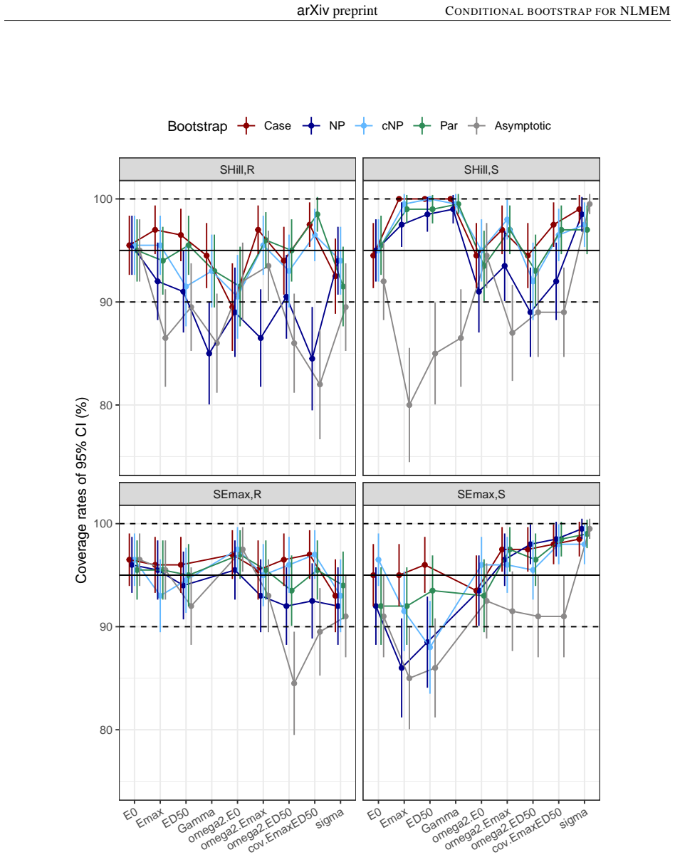
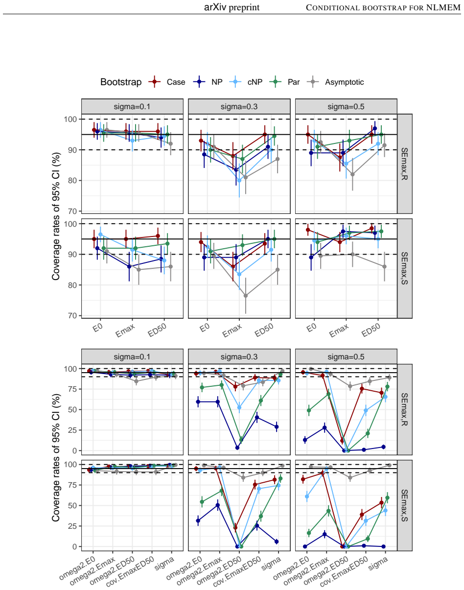
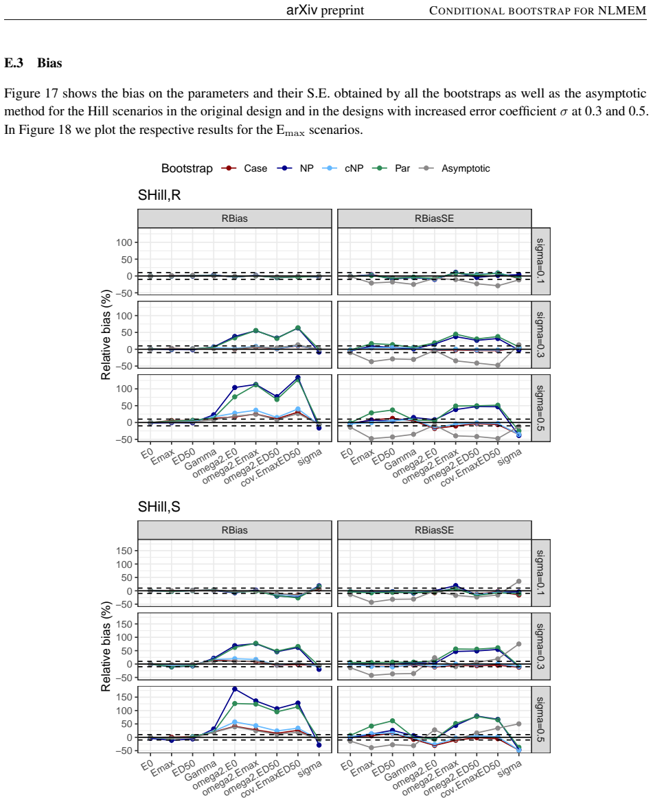
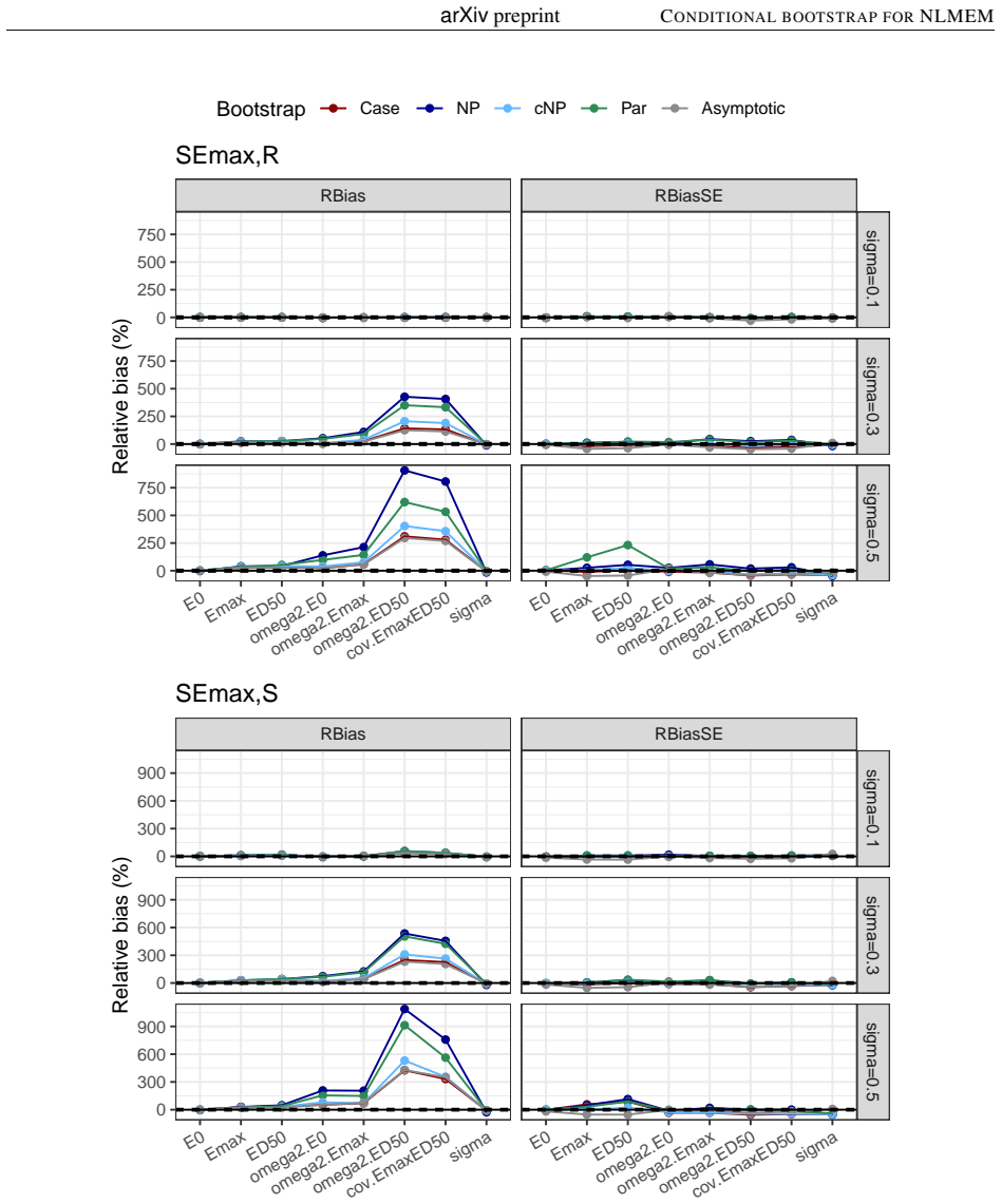
- The asymptotic method produces lower-than-nominal coverage for variance parameters across the tested designs.
- cNP maintains coverage without requiring stratification when the number of observations per subject or the covariate repartition must stay fixed.
- Both cNP and the case bootstrap outperform the classical non-parametric residual bootstrap in the reported simulations.
- All bootstrap methods lose coverage once residual variability becomes large.
- The procedure is directly available in the saemix R package for immediate use with existing SAEM fits.
Where Pith is reading between the lines
- Analysts working with sparse pharmacokinetic datasets could adopt cNP to avoid distorting subject-level observation counts when constructing confidence intervals.
- The same conditional-resampling idea might be tested in other hierarchical models whose estimation routines already produce subject-specific posterior distributions.
- Performance under non-normal random effects or more intricate covariate structures remains an open question that could be checked with targeted simulations.
- If the underlying SAEM conditional distributions themselves are misspecified, the bootstrap intervals may inherit that misspecification rather than correct it.
Load-bearing premise
The conditional distributions of the individual parameters obtained from SAEM accurately reflect the true interindividual variability without systematic bias.
What would settle it
A simulation in which the true interindividual variances are known and the empirical coverage of the cNP bootstrap intervals falls substantially below the nominal level for an unbalanced design.
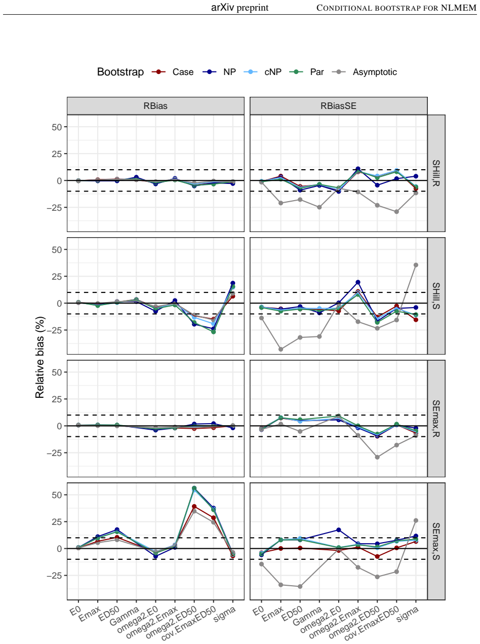
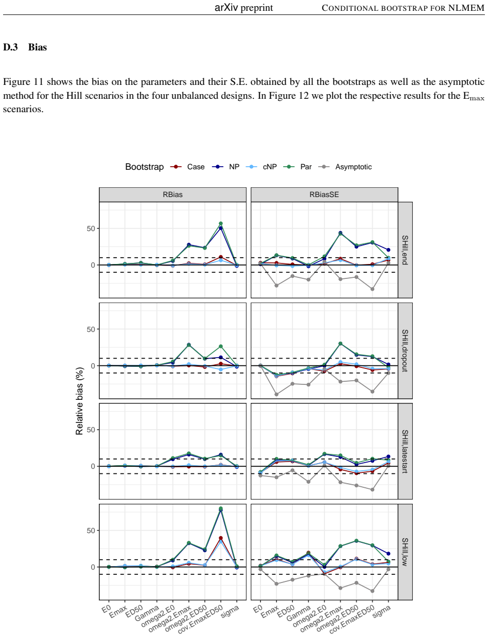
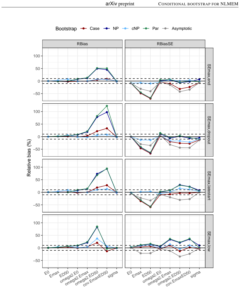
Figures


read the original abstract
Background and Objective: Uncertainty in non-linear mixed effect models is often assessed using the Fisher information matrix to derive the standard errors of estimation. The bootstrap is an alternative to the asymptotic method, with different approaches to handle the different levels of individual and population variabilities. The simplest method is the Case bootstrap where the entire vector of individuals is resampled, but this approach does not take into account the hierarchical nature of non-linear mixed effect models (NLMEM). Methods: We propose here a non-parametric bootstrap, cNP, to preserve the structure of the original data. We resample interindividual random effects from the conditional distribution of the individual parameters, obtained as a by-product of the SAEM algorithm, and residuals from their distribution. cNP was implemented in the saemix package for R along with the case, parametric (Par), and non-parametric (NP) residual bootstraps. Coverage rates were compared in a simulation study using sigmoid Emax models, with rich, sparse and unbalanced designs, and 3 levels of residual variability. Results: The asymptotic method tended to produce lower than theoretical coverages for the variance terms. Bootstraps provided more adequate coverage, but none of the approaches maintained coverage when the residual error increased. Overall, the new cNP and the Case provided better coverage than the classical NP. Conclusion: The new conditional non-parametric bootstrap can be used when it is important to preserve the structure of the original dataset, such as the number of observations or the repartition of covariates as it does not require stratification.
Editorial analysis
A structured set of objections, weighed in public.
Referee Report
Summary. The manuscript proposes a conditional non-parametric bootstrap (cNP) for non-linear mixed effects models that resamples individual random effects from the SAEM-derived conditional distributions p(η_i | y_i, θ̂) and residuals from their estimated distribution while holding the original design matrix fixed. Implemented in the saemix R package, cNP is compared to case, parametric, and classical non-parametric residual bootstraps. A simulation study using sigmoid Emax models under rich, sparse, and unbalanced designs at three residual variability levels shows that asymptotic methods undercover variance parameters, bootstraps improve coverage overall, and cNP together with case bootstrap outperform classical NP, although all methods lose coverage at high residual error. The authors conclude that cNP is suitable when preserving data structure (e.g., number of observations or covariate repartition) is required.
Significance. If the central claim holds, the work supplies a practical, structure-preserving alternative to existing bootstrap methods for NLMEM uncertainty quantification, directly addressing a common need in pharmacometrics and biostatistics. The simulation design—multiple designs, three residual levels, and explicit comparison to asymptotic and other bootstrap approaches—provides concrete, reproducible evidence of improved coverage for variance components relative to Fisher-information-based standard errors. Credit is due for the open implementation in saemix and for evaluating the method on both rich and sparse designs.
major comments (2)
- [Methods] The cNP procedure (Methods) resamples η_i from p(η_i | y_i, θ̂) evaluated at the fixed point estimate θ̂. Because the conditional distributions are not marginalized over the uncertainty in the population parameters, the resulting bootstrap distribution may be under-dispersed relative to the true sampling distribution of the NLMEM estimator. This approximation is load-bearing for the validity claim yet is not accompanied by a theoretical argument or diagnostic showing that the marginal variability is recovered; the observed coverage collapse at high residual variability could partly originate from this source.
- [Results] The simulation study (Results) reports only qualitative statements that cNP and case bootstrap achieve “better coverage” and that coverage “collapses” at high residual error. No numerical coverage rates, number of Monte Carlo replicates, exact model parameter values for the sigmoid Emax, or per-parameter coverage tables are supplied. Without these quantities it is impossible to judge the magnitude of improvement or to verify that the reported superiority is not driven by a small number of replicates or particular design realizations.
minor comments (2)
- [Abstract] The abstract states that coverage rates were compared but supplies neither the number of replicates nor any quantitative coverage figures; adding these would make the results summary self-contained.
- [Methods] Notation for the conditional distribution p(η_i | y_i, θ̂) is introduced without an explicit statement of how the SAEM by-product is extracted or whether any smoothing or kernel density estimation is applied before resampling.
Simulated Author's Rebuttal
We thank the referee for their insightful comments and the opportunity to improve our manuscript on the conditional non-parametric bootstrap for non-linear mixed effects models. We address each of the major comments in detail below, indicating the revisions we plan to make.
read point-by-point responses
-
Referee: [Methods] The cNP procedure (Methods) resamples η_i from p(η_i | y_i, θ̂) evaluated at the fixed point estimate θ̂. Because the conditional distributions are not marginalized over the uncertainty in the population parameters, the resulting bootstrap distribution may be under-dispersed relative to the true sampling distribution of the NLMEM estimator. This approximation is load-bearing for the validity claim yet is not accompanied by a theoretical argument or diagnostic showing that the marginal variability is recovered; the observed coverage collapse at high residual variability could partly originate from this source.
Authors: We recognize the validity of this observation regarding the conditional nature of our cNP procedure. By resampling from the conditional distributions p(η_i | y_i, θ̂) at the fixed θ̂, the method approximates the bootstrap distribution without fully accounting for uncertainty in the population parameters. This choice prioritizes computational efficiency and structure preservation, which is a key advantage for applications where maintaining the original data design is important. Although we do not provide a new theoretical proof of marginal coverage recovery in this work, the empirical results from our simulation study support the practical utility of cNP, showing superior coverage for variance parameters compared to asymptotic and classical NP methods in most scenarios. We agree that the coverage degradation at high residual variability may relate to this or other factors and will revise the manuscript to include an expanded discussion on the limitations of the conditional approximation, potential reasons for coverage loss, and recommendations for when cNP is most appropriate. Additional simulation diagnostics will be considered if they can be implemented without excessive computation. revision: partial
-
Referee: [Results] The simulation study (Results) reports only qualitative statements that cNP and case bootstrap achieve “better coverage” and that coverage “collapses” at high residual error. No numerical coverage rates, number of Monte Carlo replicates, exact model parameter values for the sigmoid Emax, or per-parameter coverage tables are supplied. Without these quantities it is impossible to judge the magnitude of improvement or to verify that the reported superiority is not driven by a small number of replicates or particular design realizations.
Authors: We appreciate this feedback on the presentation of our simulation results. The current manuscript emphasizes qualitative comparisons to highlight the overall trends. In the revised version, we will add detailed numerical results, including tables with coverage percentages for each model parameter across all designs and residual error levels. We will also report the number of Monte Carlo replicates performed, the precise values used for the sigmoid Emax model parameters, and per-parameter coverage breakdowns to facilitate a quantitative assessment of the improvements and to confirm the robustness of our findings. revision: yes
- A complete theoretical argument demonstrating that the conditional bootstrap fully recovers the marginal sampling distribution of the NLMEM estimator.
Circularity Check
No circularity: cNP bootstrap defined independently and evaluated externally via simulation
full rationale
The paper first specifies the cNP procedure as resampling individual random effects from the conditional distribution obtained as a by-product of SAEM, plus residual resampling, while preserving the original design matrix. This algorithmic definition stands alone. The simulation study on sigmoid Emax models (rich/sparse/unbalanced designs, three residual-variability levels) then measures coverage rates as an external performance check against known true values; coverage outcomes are not fed back to define, tune, or justify the resampling rule. No self-citation is invoked to establish uniqueness or to smuggle an ansatz; comparisons to case, parametric, and NP bootstraps rely on standard implementations. The derivation chain therefore contains no self-definitional, fitted-input, or load-bearing self-citation reductions.
Axiom & Free-Parameter Ledger
axioms (2)
- domain assumption The SAEM algorithm produces reliable estimates of the conditional distribution of individual parameters given the data.
- domain assumption Residuals can be treated as exchangeable draws from their marginal distribution for non-parametric resampling.
Reference graph
Works this paper leans on
-
[1]
Generate a bootstrap sample by resampling from the data and/or from the estimated model
-
[2]
Compute the estimates of the parameters of the model for the bootstrap sample
-
[3]
Case bootstrap (Case):This method consists of resampling with replacement the entire subjects ( ξi,yi where yi = (yi1, yi2, ...., yini)′) from the original data before modelling
Repeat steps 1-2Btimes to obtain the bootstrap distribution of the parameter estimates. Case bootstrap (Case):This method consists of resampling with replacement the entire subjects ( ξi,yi where yi = (yi1, yi2, ...., yini)′) from the original data before modelling. It is also called thepaired bootstrap. It is the most straightforward way to do bootstrapp...
-
[5]
draw a sample{η ∗ i }i=1,...,N from a normal distribution with mean zero and covariance matrix ˆΩ
-
[6]
draw a sample {ϵ∗ ij}j=1,...ni from a normal distribution with mean zero and covariance matrix Ini where I denotes the identity matrix
-
[7]
The bootstrap sample is obtained as follows:
generate the bootstrap responses y∗ ij =f(x ij,ˆµ, η∗ i ) +g(x ij,ˆµ, η∗ i , σ)ϵ ∗ ij (where we explicitly replace ψi by ˆµandη∗ i to highlight the dependency on the resampled random effects) Non-parametric residual bootstrap (NP):This method resamples with replacement from the residuals obtained after model fitting for all subjects. The bootstrap sample ...
-
[8]
fit the model to the data to obtain ˆθ
-
[9]
estimate the individual parametersˆηi as the EBE, then center and normalise them as detailed below 15 arXivpreprintCONDITIONAL BOOTSTRAP FORNLMEM
-
[10]
draw a sampleη ∗ i with replacement fori= 1, ...Nfrom the resulting set
-
[11]
calculate the residualsˆϵij =y ij −f(x ij,ˆµ,ˆηi), then center and normalise them
-
[12]
draw a sample{ϵ ∗ ij}j=1,...ni with replacement globally from the resulting set
-
[13]
To correct for this, Carpenter et al
generate the bootstrap responsesy ∗ ij =f(x ij,ˆµ, η∗ i ) +g(x ij,ˆµ, η∗ i , σ)ϵ ∗ ij The normalisation in step (b) and (d) is necessary because the EBE generally suffer from regression to the mean and their variance may be considerably smaller than the true variability in the population (Karlsson and Savic (2007)). To correct for this, Carpenter et al. (...
2007
-
[14]
center the raw estimated random effects:˜ηi = ˆηi −¯ηi
-
[15]
obtain the EVD of the estimated variance-covariance matrix: ˆΩ =V Ω DΩV T Ω where DΩ is the diagonal matrix containing the eigenvalues of ˆΩ
-
[16]
obtain the EVD of S, the variance-covariance matrix of the centered random effects: S=V S DSV T S where DS is the diagonal matrix containing the eigenvalues ofS
-
[17]
calculate the correction matrixA η using these two decompositions as Aη =V S D−1/2 S VΩ D−1/2 Ω
-
[18]
transform the centered random effects using the ratioA η:ˆη ′ i = ˜ηi ×A η Similarly, the residuals are transformed using the empirical variance:
-
[19]
center the raw estimated residuals:˜ϵij = ˆϵij −¯ϵij
-
[20]
calculate the correction factor Aσ = 1/σemp where σemp is the empirical standard deviation of the centered residuals
-
[21]
(2017)) and is avail- able on CRAN
transform the centered residuals using the ratioA σ:ˆϵ ′ ij = ˜ϵij ×A σ Implementation and runtimes The bootstrap methods were implemented for the saemix package in version 3.2 (Comets et al. (2017)) and is avail- able on CRAN. Development versions are downloadable on github https://github.com/saemixdevelopment/ saemixextension. In terms of runtimes, the ...
2017
discussion (0)
Sign in with ORCID, Apple, or X to comment. Anyone can read and Pith papers without signing in.