arxiv: 2605.04168 · v1 · submitted 2026-05-05 · 🧮 math.PR · cs.NA· math.NA

Recognition: 2 theorem links

· Lean Theorem

Error analysis for learning fractional stochastic differential equations with applications in neural approximations

Kerlyns Martinez, Lauri Viitasaari, Mahdi Dehshiri

Pith reviewed 2026-05-08 18:07 UTC · model grok-4.3

classification 🧮 math.PR cs.NAmath.NA

keywords fractional stochastic differential equationserror analysisSobolev normsnonparametric estimationneural network approximationconvergence ratesdiscrete observationsmodel fitting error

0 comments

The pith

Error analysis unifies discretization, approximation, and fitting errors for fractional SDEs using Sobolev norms that reflect trajectory regularity.

A machine-rendered reading of the paper's core claim, the machinery that carries it, and where it could break.

The authors develop a framework to analyze errors when fitting nonparametric models to fractional stochastic differential equations observed only at discrete times. They separate the total error into time discretization, coefficient approximation, and model fitting, then bound their combined effect with Sobolev-type norms that depend on how regular the trajectories are. This matters for anyone using neural networks to learn such equations because the rates show how to choose discretization and network size to make the learned model close to the true one. The framework is demonstrated on shallow neural networks with recurrent layers, and simulations back up the theory.

Core claim

The central claim is that the three primary error sources in discrete-observation nonparametric fitting of fractional SDEs can be controlled together through Sobolev-type norms, producing convergence rates that explicitly include the regularity of the solution paths and capture how the errors interact with each other.

What carries the argument

A unified error decomposition quantified via Sobolev-type norms that incorporates trajectory regularity to bound the sum of discretization, approximation, and fitting errors.

Load-bearing premise

The trajectories possess enough regularity for Sobolev norms to make sense and for the three error sources to be bounded with controlled interactions.

What would settle it

Run numerical experiments with known fractional SDEs of varying regularity, refine the discretization step and training data size, and check if the measured total error decreases at the exact rates predicted by the Sobolev norm analysis; failure to match would falsify the interaction control.

Figures

Figures reproduced from arXiv: 2605.04168 by Kerlyns Martinez, Lauri Viitasaari, Mahdi Dehshiri.

**Figure 1.** Figure 1: The drift (first row) and diffusion (second row) values for both scalar fields: the ground truth (first column) and their estimates in the 1D case. The second, third and fourth columns correspond to estimation for Hurst exponents of 0.5, 0.7 and 0.9, respectively. making diffusion-related weight updates less effective. This phenomenon is further highlighted in view at source ↗

**Figure 2.** Figure 2: The drift (first row) and diffusion (second row) values for both vector fields: the ground truth (first column) and their corresponding estimates in the 2D case. The second, third and fourth columns correspond to estimation for Hurst exponents of 0.5, 0.7 and 0.9, respectively. these contributions. During the whole experiments in this section, we fix the fine time step to ∆tfine “ 0.05, ∆tfine “ ∆tcoarse{… view at source ↗

**Figure 3.** Figure 3: Two-dimensional trajectories for the ground truth (top row) and the estimated models (bottom row). Columns correspond to H “ 0.5, H “ 0.7 and H “ 0.9, respectively. To evaluate the fitting error arising from the estimation of Hurst index H, we consider several univariate settings with a fixed number of trajectories and varying numbers of observation points M. As M increases, we expect the Hurst estimator t… view at source ↗

**Figure 4.** Figure 4: Mean and standard deviations of validation losses versus hidden-layer width in loglog-scale in 1D setting with H “ 0.7, ∆p “ 0.05, and ∆tfine “ ∆p {4. Reference slope n ´ 1 2 is shown in black. 200 400 600 800 1000 M 0.00 0.05 0.10 0.15 0.20 0.25 0.30 0.35 0.40 Error Fractional mean-error ±std Reference line ( log(M) M ) /4 for = 0.51 view at source ↗

**Figure 5.** Figure 5: Mean and standard deviations of fitting error as a function of M in 1D setting with H “ 0.7, ∆ˆ “ 0.05, ∆tfine “ ∆ˆ {4. Theoretical upper bound ´ logpMq M ¯γ{4 for γ “ 0.51 is shown in black. References [1] Avelin B., Kuusi T., Nummi P., Saksman E., Tölle J. M. & Viitasaari L. (2025). Renormalized stochastic pressure equation with log-correlated Gaussian coefficients. Journal of Differential Equations 439… view at source ↗

read the original abstract

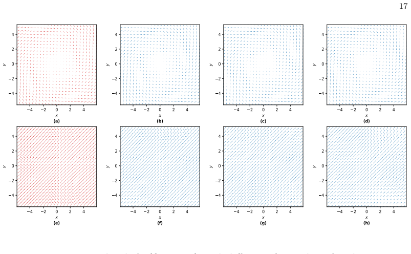
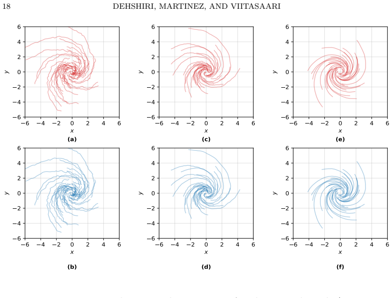
This paper develops a framework for the error analysis in nonparametric model fitting of fractional stochastic differential equations based on discrete observations. We identify and quantify the main error sources -- time discretization, coefficient approximation, and model fitting error -- within a unified framework. Through Sobolev-type norms, we derive convergence rates that incorporate the regularity of trajectories, thereby capturing the interaction of these error components. To demonstrate the applicability of the theory, we introduce a training scheme for coefficient function estimation based on shallow neural networks and a recurrent architecture. Numerical experiments validate the theoretical findings and illustrate the effectiveness of the approach.

Editorial analysis

A structured set of objections, weighed in public.

Desk editor's note, referee report, simulated authors' rebuttal, and a circularity audit. Tearing a paper down is the easy half of reading it; the pith above is the substance, this is the friction.

Desk Editor's Note private letter to a colleague

The paper unifies discretization, approximation, and fitting errors for fractional SDEs inside Sobolev norms, but the needed path regularity may not hold automatically for Hurst parameters below 1/2.

read the letter

The main thing to know is that this work puts three error sources—time discretization, coefficient approximation, and model fitting—into one Sobolev-norm framework for fractional SDEs observed at discrete times, then derives rates that depend on trajectory regularity. They follow this with a training scheme using shallow neural networks plus a recurrent architecture and some numerical checks that appear to match the rates.

Referee Report

2 major / 2 minor

Summary. The manuscript develops a framework for error analysis of nonparametric fitting for fractional SDEs observed at discrete times. It decomposes the total error into time-discretization, coefficient-approximation, and model-fitting components, then employs Sobolev-type norms to obtain convergence rates that incorporate trajectory regularity and control the interactions among the three sources. The theory is specialized to coefficient estimation via shallow neural networks and recurrent architectures, with numerical experiments offered as validation.

Significance. A rigorously justified unified rate that accounts for the interplay of discretization, approximation, and statistical errors would be a useful contribution to the analysis of learning problems for processes with memory, especially if the rates remain explicit in the Hurst parameter and mesh size. The neural-network application illustrates one concrete use case.

major comments (2)

[§3 (Error Analysis) and Assumption 2.1] The central convergence statement (presumably Theorem 3.1 or the main result in §3) invokes Sobolev norms of order s > 1/2 + d/2 to bound cross terms between discretization and approximation errors. For fractional Brownian motion with Hurst index H < 1/2 the driving noise yields paths that are only Hölder-α with α < H; the paper does not derive the necessary restriction on H (or the compensating logarithmic factor) that would make the chosen s admissible under the discrete-observation scheme.
[§3.2 and the statement of the main rate] The claim that the three error sources interact in a controlled way inside the Sobolev norm (Abstract and §3.2) rests on interpolation inequalities whose constants depend on the fractional order α and the mesh size. No explicit dependence of the final rate on α is displayed, nor is it shown that the bound remains valid when α is chosen independently of H.

minor comments (2)

[§2.1] The notation for the Sobolev norm (Eq. (2.3)) should explicitly record the underlying domain and the precise definition of the fractional derivative used.
[§5] Numerical figures would benefit from reporting the number of independent runs and standard deviations to allow assessment of variability in the neural-network training.

Simulated Author's Rebuttal

2 responses · 0 unresolved

We thank the referee for the careful reading and valuable comments on our manuscript. We address each major comment point by point below, indicating where revisions will be made to strengthen the presentation and clarify the assumptions.

read point-by-point responses

Referee: [§3 (Error Analysis) and Assumption 2.1] The central convergence statement (presumably Theorem 3.1 or the main result in §3) invokes Sobolev norms of order s > 1/2 + d/2 to bound cross terms between discretization and approximation errors. For fractional Brownian motion with Hurst index H < 1/2 the driving noise yields paths that are only Hölder-α with α < H; the paper does not derive the necessary restriction on H (or the compensating logarithmic factor) that would make the chosen s admissible under the discrete-observation scheme.

Authors: We appreciate the referee's observation on the compatibility between the Sobolev order s and the path regularity induced by fractional Brownian motion. In the error analysis of §3, the condition s > 1/2 + d/2 is imposed to invoke Sobolev embeddings that control the cross terms arising from the decomposition into discretization, approximation, and fitting errors. Assumption 2.1 encodes the regularity of the coefficients and the driving noise, but does not yet explicitly link this to the admissible range of H. We will revise the statement of the main result (Theorem 3.1) by adding a remark that explicitly requires H > 1/2 + d/2 (ensuring the Hölder exponent α exceeds s) for the stated rate to hold without logarithmic corrections. When H is smaller, we will note that a mild logarithmic factor in the mesh size can be absorbed into the bound, consistent with standard Hölder regularity results for fBM. This revision will also confirm compatibility with the discrete-observation scheme. revision: yes
Referee: [§3.2 and the statement of the main rate] The claim that the three error sources interact in a controlled way inside the Sobolev norm (Abstract and §3.2) rests on interpolation inequalities whose constants depend on the fractional order α and the mesh size. No explicit dependence of the final rate on α is displayed, nor is it shown that the bound remains valid when α is chosen independently of H.

Authors: We agree that the interpolation inequalities employed in §3.2 to bound the interactions among the three error sources have constants that depend on the fractional order α and the mesh size. In the current version these dependencies are absorbed into generic constants appearing in the convergence rate. We will revise the main rate statement to display the explicit dependence on α. We will also add a clarifying paragraph in §3.2 explaining that α is determined by the Hurst parameter H via the Hölder regularity of the driving noise, yet the underlying interpolation bounds remain valid for any fixed α satisfying the necessary inequalities (with s chosen relative to α), even when α is selected independently of the specific value of H. This will make the generality of the framework transparent. revision: yes

Circularity Check

0 steps flagged

No significant circularity; derivation self-contained from regularity assumptions

full rationale

The paper presents a theoretical framework deriving convergence rates for error components in fractional SDE model fitting via Sobolev-type norms applied to trajectory regularity. No steps reduce by construction to fitted parameters, self-citations, or renamed inputs; the bounds follow from standard embedding and interpolation inequalities under stated regularity. The analysis identifies three error sources and controls their interactions directly from the assumed Sobolev index without redefining quantities in terms of the target rates. External benchmarks (numerical validation) are separate from the derivation chain. This is the expected non-finding for a pure error-analysis paper.

Axiom & Free-Parameter Ledger

0 free parameters · 0 axioms · 0 invented entities

Abstract provides no explicit free parameters, axioms, or invented entities; full manuscript required to audit any hidden assumptions on fractional orders or observation models.

pith-pipeline@v0.9.0 · 5399 in / 961 out tokens · 29077 ms · 2026-05-08T18:07:30.438842+00:00 · methodology

discussion (0)

Reference graph

Works this paper leans on

29 extracted references · 1 canonical work pages

[1]

Avelin B., Kuusi T., Nummi P., Saksman E., Tölle J. M. & Viitasaari L. (2025).Renormalized stochastic pressure equation with log-correlated Gaussian coefficients.Journal of Differential Equations 439, 113416. 20 DEHSHIRI, MARTINEZ, AND VIITASAARI

2025
[2]

& Gatheral J

Bayer C., Friz P. & Gatheral J. (2016).Pricing under rough volatility.Quantitative Finance 16(6), 887–904

2016
[3]

& Scholes M

Black F. & Scholes M. (1973).The pricing of options and corporate liabilities.Journal of political economy 81(3), 637–654

1973
[4]

& Maurer P

Bossy M., Martinez K. & Maurer P. (2025).Weak rough kernel comparison via PPDEs for integrated Volterra processes.arXiv preprint arXiv:2501.07509

work page arXiv 2025
[5]

& Scotti S

Bondi A., Pulido S. & Scotti S. (2024).The rough Hawkes Heston stochastic volatility model. Mathematical Finance 34(4), 1197–1241

2024
[6]

Chen R. T. Q., Rubanova Y., Bettencourt J. & Duvenaud D. K. (2018).Neural ordinary differential equations.Advances in Neural Information Processing Systems 31

2018
[7]

(2001).Estimating the parameters of a fractional Brownian motion by discrete variations of its sample paths.Statistical Inference for Stochastic Processes 4(2), 199–227

Coeurjolly J.-F. (2001).Estimating the parameters of a fractional Brownian motion by discrete variations of its sample paths.Statistical Inference for Stochastic Processes 4(2), 199–227

2001
[8]

The Journal of Computational Finance 7, 1–49

ContR.&TankovP.(2004).Nonparametric calibration of jump-diffusion option pricing models. The Journal of Computational Finance 7, 1–49

2004
[9]

(2012).A Milstein-type scheme without Lévy area terms for SDEs driven by fractional Brownian motion

Deya A., Neuenkirch A., & Tindel S. (2012).A Milstein-type scheme without Lévy area terms for SDEs driven by fractional Brownian motion. Annales de l’IHP Probabilités et statistiques, 48(2), 518–550

2012
[10]

& Nakagawa K

Hayashi K. & Nakagawa K. (2022).Fractional SDE-Net: Generation of time series data with long-term memory.IEEE 9th International Conference on Data Science and Advanced Ana- lytics (DSAA), 1–10

2022
[11]

(2023).Variability of paths and differential equations with BV-coefficients

Hinz M., Tölle J., & Viitasaari L. (2023).Variability of paths and differential equations with BV-coefficients. Annales de l’Institut Henri Poincare (B) Probabilites et statistiques, 59(4), 2036–2082

2023
[12]

& Auer P

Hornik K., Stinchcombe M., White H. & Auer P. (1994).Degree of approximation results for feedforward networks approximating unknown mappings and their derivatives.Neural compu- tation, 6(6), 1262-1275

1994
[13]

& Nualart D

Hu Y., Liu Y. & Nualart D. (2016).Rate of convergence and asymptotic error distribution of Euler approximation schemes for fractional diffusions. The Annals of Applied Probability, 26(2), 1147–1207

2016
[14]

& Nualart D

Hu Y. & Nualart D. (2010).Parameter estimation for fractional Ornstein–Uhlenbeck processes. Statistics & Probability Letters 80(11-12), 1030–1038

2010
[15]

& Nualart D

Hu Y. & Nualart D. (2010).Differential equations driven by Hölder continuous functions of order greater than 1/2.Stochastic Analysis and Applications: The Abel Symposium 2005. Springer Berlin Heidelberg, 2007

2010
[16]

& Lyons T

Kidger P., Foster J., Li X. & Lyons T. J. (2021).Neural SDEs as infinite-dimensional GANs. In: International Conference on Machine Learning, 5453–5463

2021
[17]

& Ralchenko K

Kubilius K., Mishura Y. & Ralchenko K. (2017).Parameter Estimation in Fractional Diffusion Models.Bocconi & Springer Series, 8: Mathematics, Statistics, Finance and Economics

2017
[18]

Kutz J. N. (2017).Deep learning in fluid dynamics.Journal of Fluid Mechanics 814, 1–4

2017
[19]

Mandelbrot B. B. & Van Ness J. W. (1968).Fractional Brownian motions, fractional noises and applications.SIAM Review 10(4), 422–437

1968
[20]

& Shevchenko G

Mishura Y. & Shevchenko G. (2008).The rate of convergence for Euler approximations of solutions of stochastic differential equations driven by fractional Brownian motion.Stochastics An International Journal of Probability and Stochastic Processes, 80(5), 489–511

2008
[21]

& Răşcanu A.(2002).Differential equations driven by fractional Brownian motion

Nualart D. & Răşcanu A.(2002).Differential equations driven by fractional Brownian motion. Collectanea Mathematica, 53(1), 55–81

2002
[22]

& Viitasaari L

Nummi P. & Viitasaari L. (2024).Necessary and sufficient conditions for continuity of hyper- contractive processes and fields.Statistics & Probability Letters, 208, 110049

2024
[23]

Pope S. B. (1994).On the relationship between stochastic Lagrangian models of turbulence and second-moment closures.Physics of Fluids 6(2), 973–985. 21

1994
[24]

& Viitasaari L

Shevchenko G. & Viitasaari L. (2015).Adapted integral representations of random variables. Int. J. Mod. Phys. Conf. Ser. 36

2015
[25]

Foundations of Computational Mathematics, 24(2), 481-537

SiegelJ.&XuJ.(2024).Sharp bounds on the approximation rates, metric entropy, andn-widths of shallow neural networks. Foundations of Computational Mathematics, 24(2), 481-537

2024
[26]

& Zeng C

Viitasaari L. & Zeng C. (2022).Stationary Wong–Zakai Approximation of Fractional Brownian Motion and Stochastic Differential Equations with Noise Perturbations. Fractal and Fractional, 6(6), 303

2022
[27]

& Hlubinka D

Štěpán J. & Hlubinka D. (2007).Kermack-McKendrick epidemic model revisited.Kybernetika 43(4), 395–414

2007
[28]

YangL., GaoT., LuY., DuanJ.&LiuT.(2023).Neural network stochastic differential equation models with applications to financial data forecasting.Applied Mathematical Modelling 115, 279–299

2023
[29]

ˆ t´s ´8 ! pt´s´rq H1´1{2 ´ p´rqH1´1{2 ` ) ! pt´s´rq H2´1{2 ´ p´rqH2´1{2 ` ) dr “ pt´sq H1`H2 ˆ 8 ´1 ! p1`uq H1´1{2 ´u H1´1{2 ` ) ! p1`uq H2´1{2 ´u H2´1{2 ` ) du “ |t´s| H1`H2

Yarotsky D. (2017).Error bounds for approximations with deep ReLU networks. Neural net- works, 94, 103-114. Appendix A. Proof of Theorem 2.2 We split the proof into a series of lemmas and three propositions dealing with different sources of error. We begin with the time-discretisation error that follows directly from the existing results presented in the ...

2017