Recognition: unknown
The Demand Externality of Automation
Pith reviewed 2026-05-08 16:05 UTC · model grok-4.3
The pith
Firms may choose too much automation when it cuts income for high-MPC low-wealth households while ownership stays concentrated.
A machine-rendered reading of the paper's core claim, the machinery that carries it, and where it could break.
Core claim
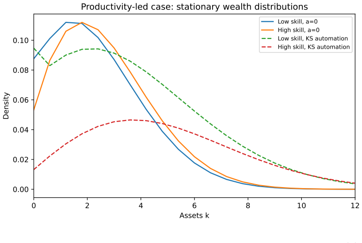
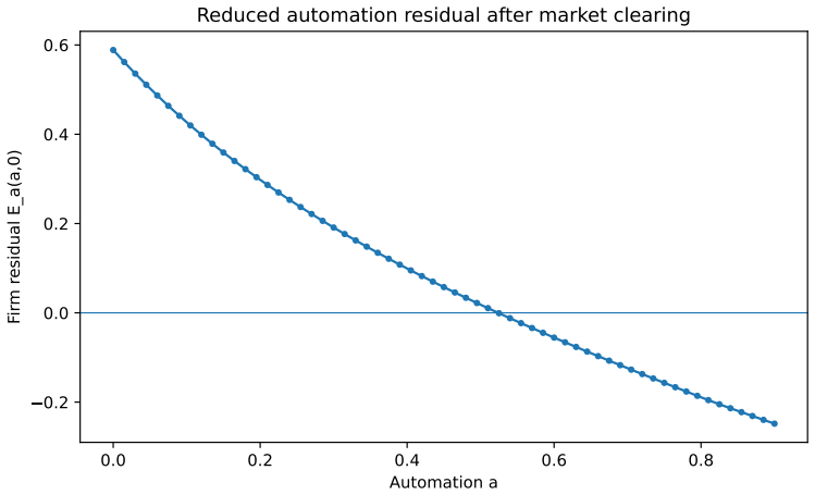
Automation is chosen by profit-maximizing firms from a production function that trades off labor savings against capital costs. In the stationary equilibrium, wages and returns clear markets under Cobb-Douglas technology, while the wealth distribution evolves according to households' optimal saving rules. The paper identifies the externality as the derivative of aggregate consumption demand with respect to automation: this derivative is negative when automation reduces the wage bill paid to high-MPC households more than it raises capital income for low-MPC owners. Under these conditions, equilibrium automation is excessive even though high-skilled labor income rises.
What carries the argument
The derivative of household consumption demand and the aggregate wage bill with respect to the automation parameter, which measures the uninternalized demand effect under incomplete insurance and heterogeneous marginal propensities to consume.
If this is right
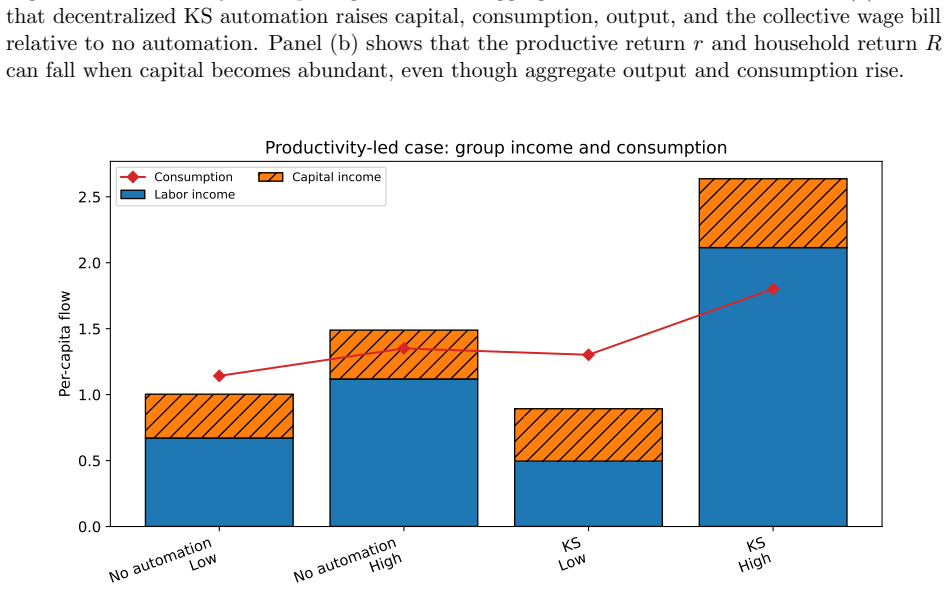
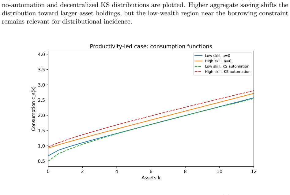
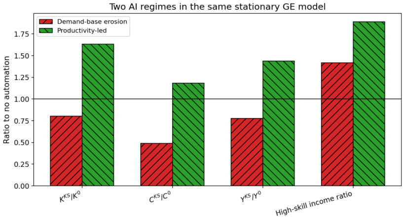
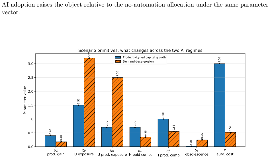
- With broad ownership and strong high-skill complementarity, automation raises output, capital stock, and consumption for all groups.
- When ownership is concentrated and low-wealth households bear most labor-income losses, private automation exceeds the level that maximizes total consumption.
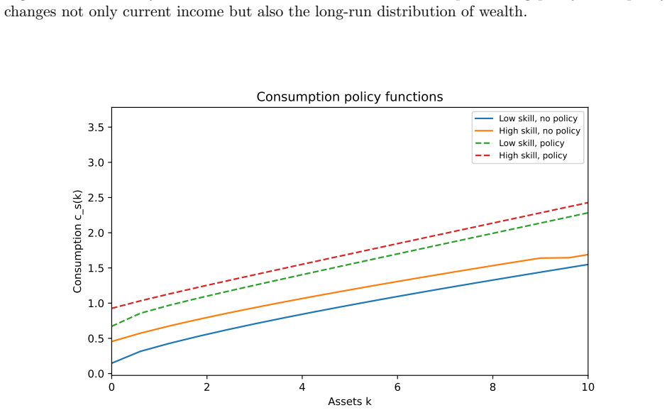
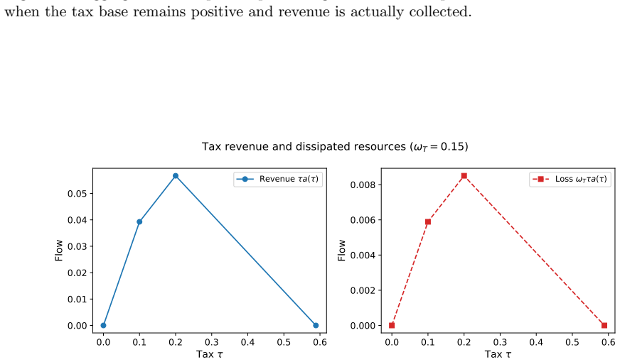
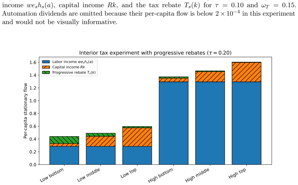
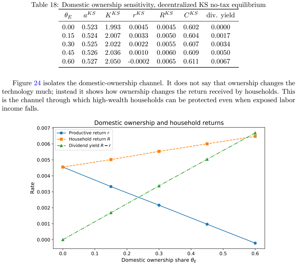
- A tax on automation that modifies the firm's first-order condition can raise revenue while shifting the equilibrium toward the social optimum, with rebates distributed according to the same ownership pattern.
- The size of the externality depends on the degree of wealth inequality and the strength of the link between automation and labor demand for high-MPC workers.
Where Pith is reading between the lines
- In economies where automation substitutes mainly for routine tasks performed by middle-wealth workers, the demand externality could be smaller than in the model's low-wealth focus.
- Extending the framework to allow endogenous skill acquisition would test whether the externality persists when workers can respond to automation by changing their skill composition.
- The same mechanism implies that subsidies for automation without accompanying redistribution may amplify short-run demand shortfalls in high-inequality settings.
Load-bearing premise
Households cannot fully insure against the income losses automation imposes on low-wealth groups, so their consumption falls more than high-wealth owners' consumption rises.
What would settle it
Removing differences in marginal propensities to consume across wealth levels, or introducing complete insurance markets that let all households smooth income perfectly, should eliminate any gap between private and socially optimal automation in the model.
Figures


read the original abstract
Automation raises productivity and reduces paid human labor, but it also reallocates income and ownership claims. This paper studies that tradeoff in a static benchmark and in a stationary heterogeneous-agent general equilibrium. Firms choose automation from a profit function. Households differ by skill and wealth, save in a capital/equity claim, and face incomplete insurance. Wages and returns are determined by market clearing from a Cobb--Douglas final-good firm, while the wealth distribution is pinned down by a Hamilton--Jacobi--Bellman (HJB) equation and a Kolmogorov forward equation (KFE). The paper is deliberately two-sided. With strong productivity growth, high-skill complementarity, low obsolescence, and broad ownership, automation raises output, capital, and consumption. With strong exposure of low-wealth, high-marginal-propensity-to-consume (high-MPC) households and concentrated ownership, privately chosen automation can be excessive even though it raises high-skilled labor income. The central object is the derivative of household consumption demand and collective wage bill with respect to automation. Fiscal policy is modeled as a government problem rather than as an abstract planner: a tax changes the firm's automation first-order condition, raises revenue only on the remaining automation base, and must specify rebates and administrative losses.
Editorial analysis
A structured set of objections, weighed in public.
Referee Report
Summary. The paper studies the demand externality of automation in a static benchmark and a stationary heterogeneous-agent general equilibrium with incomplete insurance markets. Firms choose automation to maximize profits under Cobb-Douglas production with skill complementarity. Households differ by skill and wealth, save in a capital/equity claim, and the wealth distribution is determined by an HJB equation and KFE. The analysis is two-sided: under high productivity growth, high-skill complementarity, low obsolescence, and broad ownership, automation raises output, capital, and consumption; under strong exposure of low-wealth high-MPC households and concentrated ownership, privately optimal automation exceeds the social optimum due to a negative externality identified as the derivative of household consumption demand and the wage bill with respect to automation, even as high-skilled labor income rises. Fiscal policy is modeled via a tax that shifts the firm's automation FOC, with revenue raised only on the remaining base and specified rebates.
Significance. If the central externality result holds after verification, the paper makes a valuable contribution to the literature on automation, technological change, and inequality by providing a mechanism through which private firm decisions can generate excessive automation in incomplete-markets economies with heterogeneous MPCs and ownership. The deliberate two-sided comparative statics are a strength, as is the use of continuous-time HA methods to endogenize the wealth distribution. This framework could support policy analysis of automation taxes. The approach is grounded in standard tools (profit FOC, HJB/KFE) and offers falsifiable predictions about when automation is welfare-improving versus excessive.
major comments (2)
- [Stationary GE] In the stationary heterogeneous-agent GE section, the central claim that privately chosen automation is excessive rests on the derivative of aggregate consumption demand and the wage bill with respect to automation correctly proxying the social marginal welfare effect. However, because automation shifts the entire stationary wealth distribution via the KFE (and thereby alters marginal utilities, insurance properties of the equity claim, and consumption across heterogeneous agents), it must be shown explicitly whether this derivative is computed holding the distribution fixed or fully incorporating the endogenous distributional response; otherwise the identification of a negative demand externality does not follow from the primitives.
- [Fiscal policy] In the fiscal policy modeling, the government problem is specified as a tax that alters the firm's automation first-order condition with revenue collected only on the post-tax automation base. The welfare comparison to the social optimum requires a complete statement of how tax revenue is rebated (e.g., lump-sum to which households) and how any administrative losses enter the government budget; without these details the policy implications for correcting the externality cannot be assessed.
minor comments (2)
- [Model setup] The notation for the skill-complementarity parameter and the obsolescence rate in the production function should be defined explicitly at first use to make the two-sided comparative statics easier to follow.
- [Introduction] The abstract and introduction refer to 'strong exposure of low-wealth, high-MPC households'; a brief table or figure summarizing the calibrated or assumed MPCs by wealth quintile would improve readability.
Simulated Author's Rebuttal
We thank the referee for the constructive and detailed comments. We address each major point below and indicate the revisions we will make to strengthen the paper.
read point-by-point responses
-
Referee: [Stationary GE] In the stationary heterogeneous-agent GE section, the central claim that privately chosen automation is excessive rests on the derivative of aggregate consumption demand and the wage bill with respect to automation correctly proxying the social marginal welfare effect. However, because automation shifts the entire stationary wealth distribution via the KFE (and thereby alters marginal utilities, insurance properties of the equity claim, and consumption across heterogeneous agents), it must be shown explicitly whether this derivative is computed holding the distribution fixed or fully incorporating the endogenous distributional response; otherwise the identification of a negative demand externality does not follow from the primitives.
Authors: We thank the referee for this important clarification request. In the current manuscript the derivative is evaluated at the stationary equilibrium, which is obtained by jointly solving the HJB and KFE so that the full endogenous distributional response is already embedded. The negative demand externality is therefore the total (not partial) effect. To make this transparent we will add an explicit decomposition in the revised text: the direct partial derivative holding the wealth distribution fixed, plus the indirect effect operating through the KFE-induced shifts in marginal utilities and consumption. This decomposition will confirm that the externality remains negative after the distributional adjustment, driven by the disproportionate impact on high-MPC low-wealth households under concentrated ownership. revision: yes
-
Referee: [Fiscal policy] In the fiscal policy modeling, the government problem is specified as a tax that alters the firm's automation first-order condition with revenue collected only on the post-tax automation base. The welfare comparison to the social optimum requires a complete statement of how tax revenue is rebated (e.g., lump-sum to which households) and how any administrative losses enter the government budget; without these details the policy implications for correcting the externality cannot be assessed.
Authors: We agree that the fiscal-policy section needs fuller specification to support welfare comparisons. In the revision we will state explicitly that tax revenue is rebated as equal lump-sum transfers to every household (independent of skill or current wealth) and that the government budget is balanced with zero administrative losses. With these details added, the tax-adjusted equilibrium can be directly compared to the social optimum, clarifying the policy implications. revision: yes
Circularity Check
No significant circularity; derivation uses standard primitives
full rationale
The paper constructs a heterogeneous-agent model with explicit Cobb-Douglas production, HJB value function for households, and KFE for the stationary wealth distribution. The central externality object is computed directly as the derivative of aggregate consumption demand and wage bill with respect to the automation choice variable inside this solved equilibrium. No step reduces a prediction to a fitted parameter by construction, nor does any load-bearing claim rest on a self-citation chain or imported uniqueness theorem. Functional forms and market-clearing conditions are stated as modeling choices rather than derived from the target result. The analysis therefore remains self-contained against external benchmarks.
Axiom & Free-Parameter Ledger
free parameters (3)
- productivity growth
- skill complementarity
- obsolescence rate
axioms (3)
- standard math Cobb-Douglas final-good production
- domain assumption Incomplete insurance markets
- domain assumption Stationary wealth distribution via HJB and KFE
Reference graph
Works this paper leans on
-
[1]
Acemoglu, D. (2008). Introduction to Modern Economic Growth. Princeton University Press
2008
-
[2]
Acemoglu, D. and P. Restrepo (2018). Artificial intelligence, automation and work. NBER Working Paper 24196
2018
-
[3]
Acemoglu, D. and P. Restrepo (2019). Automation and new tasks: How technology displaces and reinstates labor. Journal of Economic Perspectives 33(2), 3--30
2019
-
[4]
Han, J.-M
Achdou, Y., J. Han, J.-M. Lasry, P.-L. Lions, and B. Moll (2022). Income and wealth distribution in macroeconomics: A continuous-time approach. Review of Economic Studies 89(1), 45--86
2022
-
[5]
Aiyagari, S. R. (1994). Uninsured idiosyncratic risk and aggregate saving. Quarterly Journal of Economics 109(3), 659--684
1994
-
[6]
Arrow, K. J. and G. Debreu (1954). Existence of an equilibrium for a competitive economy. Econometrica 22(3), 265--290
1954
-
[7]
Rognlie, and L
Auclert, A., M. Rognlie, and L. Straub (2024). The intertemporal Keynesian cross. Journal of Political Economy 132(12), 4068--4121
2024
-
[8]
Bewley, T. (1986). Stationary monetary equilibrium with a continuum of independently fluctuating consumers. In W. Hildenbrand and A. Mas-Colell (eds.), Contributions to Mathematical Economics in Honor of Gerard Debreu. North-Holland
1986
-
[9]
Distributional Financial Accounts
Board of Governors of the Federal Reserve System (2026). Distributional Financial Accounts. https://www.federalreserve.gov/releases/z1/dataviz/dfa/distribute/chart/
2026
-
[10]
Falk, B. H. and G. Tsoukalas (2026). The AI layoff trap. Working paper
2026
-
[11]
Generative AI could raise global GDP by 7 percent
Goldman Sachs Research (2023). Generative AI could raise global GDP by 7 percent. Research note. https://www.goldmansachs.com/insights/articles/generative-ai-could-raise-global-gdp-by-7-percent
2023
-
[12]
How will AI affect the U.S
Goldman Sachs Research (2026). How will AI affect the U.S. labor market? Research note. https://www.goldmansachs.com/insights/articles/how-will-ai-affect-the-us-labor-market
2026
-
[13]
Gu, Z., M. Lauri\`ere, S. Merkel, and J. Payne (2024). Global solutions to master equations for continuous time heterogeneous agent macroeconomic models. arXiv:2406.13726. https://arxiv.org/abs/2406.13726
-
[14]
Hicks, J. R. (1932). The Theory of Wages. Macmillan
1932
-
[15]
Huggett, M. (1993). The risk-free rate in heterogeneous-agent incomplete-insurance economies. Journal of Economic Dynamics and Control 17(5--6), 953--969
1993
-
[16]
AI will transform the global economy
International Monetary Fund (2024). AI will transform the global economy. Let's make sure it benefits humanity. IMF Blog. https://www.imf.org/en/blogs/articles/2024/01/14/ai-will-transform-the-global-economy-lets-make-sure-it-benefits-humanity
2024
-
[17]
Kaplan, G. and G. L. Violante (2014). A model of the consumption response to fiscal stimulus payments. Econometrica 82(4), 1199--1239
2014
-
[18]
Moll, and G
Kaplan, G., B. Moll, and G. L. Violante (2018). Monetary policy according to HANK. American Economic Review 108(3), 697--743
2018
-
[19]
Krusell, P. and A. A. Smith (1998). Income and wealth heterogeneity in the macroeconomy. Journal of Political Economy 106(5), 867--896
1998
-
[20]
Mas-Colell, A., M. D. Whinston, and J. R. Green (1995). Microeconomic Theory. Oxford University Press
1995
-
[21]
The economic potential of generative AI: The next productivity frontier
McKinsey Global Institute (2023). The economic potential of generative AI: The next productivity frontier. https://www.mckinsey.com/capabilities/tech-and-ai/our-insights/the-economic-potential-of-generative-ai-the-next-productivity-frontier
2023
-
[22]
The state of AI: Global survey 2025
McKinsey QuantumBlack (2025). The state of AI: Global survey 2025. https://www.mckinsey.com/capabilities/quantumblack/our-insights/the-state-of-ai
2025
-
[23]
Which U.S
Pew Research Center (2023). Which U.S. workers are more exposed to AI on their jobs? https://www.pewresearch.org/social-trends/2023/07/26/which-u-s-workers-are-more-exposed-to-ai-on-their-jobs/
2023
-
[24]
The 2025 AI Index Report
Stanford Institute for Human-Centered Artificial Intelligence (2025). The 2025 AI Index Report. https://hai.stanford.edu/ai-index/2025-ai-index-report
2025
-
[25]
Tobin, J. (1969). A general equilibrium approach to monetary theory. Journal of Money, Credit and Banking 1(1), 15--29
1969
-
[26]
Bureau of Labor Statistics (2025)
U.S. Bureau of Labor Statistics (2025). Education pays, 2024. Career Outlook. https://www.bls.gov/careeroutlook/2025/data-on-display/education-pays.htm
2025
-
[27]
Treasury (2025)
U.S. Treasury (2025). Foreign portfolio holdings of U.S. securities as of June 30, 2024. Treasury International Capital report. https://ticdata.treasury.gov/resource-center/data-chart-center/tic/Documents/shl2024r.pdf
2025
discussion (0)
Sign in with ORCID, Apple, or X to comment. Anyone can read and Pith papers without signing in.