Recognition: unknown
Numerical Analysis of Space-Time Dependent Source Identification in Subdiffusion Equations
Pith reviewed 2026-05-08 07:12 UTC · model grok-4.3
The pith
A fixed-point algorithm reconstructs space-time dependent sources in subdiffusion equations from lateral boundary measurements with linear convergence and explicit error bounds.
A machine-rendered reading of the paper's core claim, the machinery that carries it, and where it could break.
Core claim
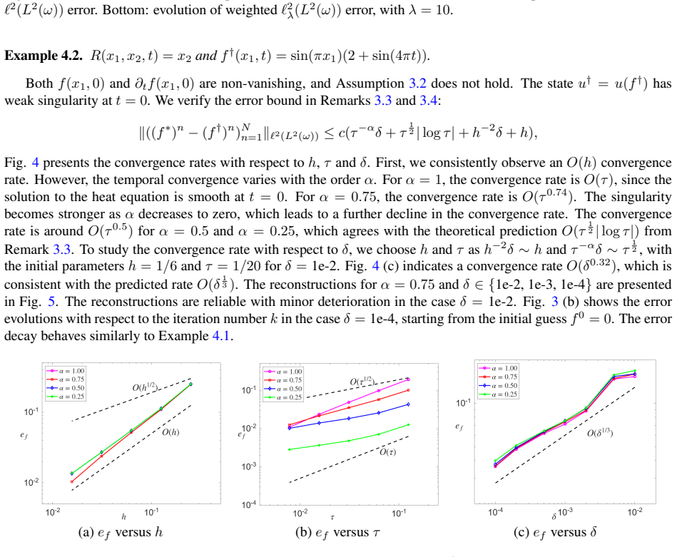
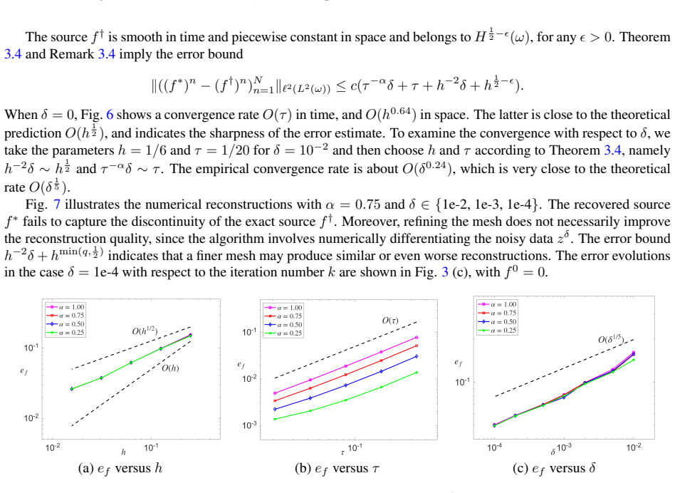
The authors introduce a fixed-point algorithm for recovering the space-time source term in a subdiffusion model from lateral boundary measurements. The scheme discretizes space with Galerkin finite elements and time with finite differences. They prove linear convergence of the iteration and obtain an a priori error bound that depends explicitly on the discretization parameters and the noise level in the data. The analysis uses the stability of the underlying continuous inverse problem together with regularity estimates for the direct problem.
What carries the argument
The fixed-point iteration that updates the source estimate by solving the direct subdiffusion problem and adjusting the source based on the boundary mismatch.
If this is right
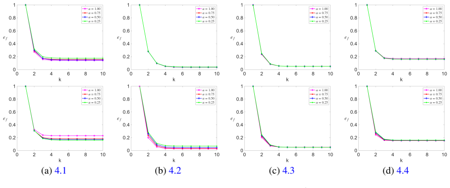
- The reconstructed source converges linearly to the true source as the iteration proceeds.
- The total error decreases when the spatial and temporal meshes are refined or when noise is reduced.
- The approach works even when the data has limited regularity.
- Numerical experiments validate the predicted convergence rates.
Where Pith is reading between the lines
- Similar fixed-point schemes might apply to other inverse problems involving fractional-order equations.
- The explicit dependence on discretization parameters could guide adaptive mesh refinement strategies in implementation.
- Testing the algorithm on real experimental data from subdiffusive systems would validate its practical utility beyond synthetic tests.
Load-bearing premise
Stability estimates hold for the continuous source identification problem and for the direct problem with rough data.
What would settle it
Run the fixed-point iteration on a manufactured solution with a known source and check whether the iteration error decreases linearly while the total reconstruction error scales with the predicted dependence on mesh size and noise level.
Figures


read the original abstract
In this work, we propose an easy-to-implement fixed-point algorithm for reconstructing a space-time dependent source in a subdiffusion model from lateral boundary measurements. The numerical scheme combines a Galerkin finite element method for spatial discretization with a finite difference method for temporal discretization. We establish the linear convergence of the fixed-point iteration and derive an error bound that depends explicitly on the discretization parameters and the noise level. The error analysis relies on stability properties of the continuous inverse problem and technical estimates for the associated direct problem with limited-regularity data. Numerical experiments are presented to support and complement the theoretical analysis.
Editorial analysis
A structured set of objections, weighed in public.
Referee Report
Summary. The paper proposes an easy-to-implement fixed-point algorithm to reconstruct a space-time dependent source in a subdiffusion equation from lateral boundary measurements. The numerical scheme uses a Galerkin finite element method in space combined with finite differences in time. Linear convergence of the fixed-point iteration is established and an explicit error bound is derived in terms of the discretization parameters and noise level. The analysis relies on stability properties of the continuous inverse problem together with a priori estimates for the direct problem under limited-regularity data. Numerical experiments are presented to support the theory.
Significance. If the assumed stability of the continuous inverse problem and the direct-problem estimates hold with constants independent of the discretization parameters and the fractional order, the work supplies a practical reconstruction method with explicit, implementable error control for an important class of inverse problems in anomalous diffusion. The combination of a simple iteration with a fully discrete scheme and the explicit dependence on noise and mesh sizes would be a useful contribution to the numerical analysis literature on fractional inverse problems.
major comments (1)
- [Error analysis / convergence theorem] The error analysis (as described in the abstract and the skeptic note) rests on stability properties of the continuous inverse problem and technical a-priori estimates for the direct subdiffusion problem with limited-regularity data. No independent verification or explicit statement of these stability constants is provided in the given description; because subdiffusion solutions generically lose regularity at t=0, these constants can depend on the fractional order α and may deteriorate near the initial time. If the stability constant grows with the noise level or depends on the discretization, the claimed explicit error bound no longer controls the total error as asserted.
minor comments (1)
- [Abstract] The abstract states that the error bound 'depends explicitly on the discretization parameters and the noise level,' but does not indicate whether the hidden constants are independent of α; this should be clarified in the statement of the main theorem.
Simulated Author's Rebuttal
We thank the referee for the careful reading and constructive feedback. We address the major comment on the error analysis below and will revise the manuscript accordingly to improve clarity.
read point-by-point responses
-
Referee: [Error analysis / convergence theorem] The error analysis (as described in the abstract and the skeptic note) rests on stability properties of the continuous inverse problem and technical a-priori estimates for the direct subdiffusion problem with limited-regularity data. No independent verification or explicit statement of these stability constants is provided in the given description; because subdiffusion solutions generically lose regularity at t=0, these constants can depend on the fractional order α and may deteriorate near the initial time. If the stability constant grows with the noise level or depends on the discretization, the claimed explicit error bound no longer controls the total error as asserted.
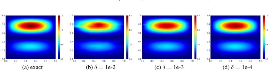
Authors: We appreciate the referee highlighting this foundational aspect. The stability of the continuous inverse problem is established with a constant depending only on the spatial domain, time interval, and α (bounded for α in any compact subinterval of (0,1)), independent of discretization parameters and noise level. The a priori estimates for the direct problem with limited regularity employ weighted spaces to control the t=0 singularity, yielding constants uniform in h and τ. The convergence theorem derives an explicit bound in which the total error is controlled by the sum of the noise term and discretization errors, with the overall constant independent of the noise level and mesh parameters. While the abstract summarizes at a high level, the full analysis verifies these properties. We agree a more explicit statement would help and will add a remark after the main error theorem clarifying the independence from h, τ, and noise, plus a brief discussion of α-dependence. revision: yes
Circularity Check
No significant circularity; derivation relies on external stability results and standard discretizations
full rationale
The paper proposes a fixed-point algorithm combining Galerkin FEM and finite differences, then claims to establish linear convergence and an explicit error bound. The abstract explicitly states that the error analysis relies on stability properties of the continuous inverse problem and technical estimates for the direct problem with limited-regularity data. These are treated as inputs from the continuous setting rather than being redefined or fitted inside the numerical scheme. No self-definitional loops, fitted inputs renamed as predictions, or load-bearing self-citations appear in the provided description. The central claims remain independent of any internal redefinition of the target quantities.
Axiom & Free-Parameter Ledger
axioms (2)
- domain assumption Stability properties of the continuous inverse problem hold
- domain assumption Technical estimates exist for the direct problem with limited-regularity data
Reference graph
Works this paper leans on
-
[1]
E. E. Adams and L. W. Gelhar. Field study of dispersion in a heterogeneous aquifer: 2. spatial moments analysis. Water Res. Research, 28(12):3293–3307, 1992
1992
-
[2]
S. C. Brenner and L. R. Scott.The Mathematical Theory of Finite Element Methods. Springer, New York, third edition, 2008
2008
-
[3]
S. Cen, B. Jin, Q. Quan, and Z. Zhou. Numerical analysis of unsupervised learning approaches for parameter identification in PDEs.Handbook of Numerical Analysis, Vol. 27, page in press, 2025
2025
-
[4]
Z. Chen, W. Zhang, and J. Zou. Stochastic convergence of regularized solutions and their finite element approx- imations to inverse source problems.SIAM J. Numer. Anal., 60(2):751–780, 2022
2022
-
[5]
D. A. Di Pietro and A. Ern.Mathematical Aspects of Discontinuous Galerkin Methods.Berlin: Springer, 2012
2012
-
[6]
H. W. Engl, M. Hanke, and A. Neubauer.Regularization of Inverse Problems. Kluwer Academic, Dordrecht, 1996
1996
-
[7]
Fujishiro and Y
K. Fujishiro and Y . Kian. Determination of time dependent factors of coefficients in fractional diffusion equa- tions.Math. Control Relat. Fields, 6(2):251–269, 2016
2016
-
[8]
Gaitan and Y
P. Gaitan and Y . Kian. A stability result for a time-dependent potential in a cylindrical domain.Inverse Problems, 29(6):065006, 18 pp., 2013
2013
-
[9]
Grisvard.Elliptic Problems in Nonsmooth Domains
P. Grisvard.Elliptic Problems in Nonsmooth Domains. Pitman, Boston, MA, 1985
1985
-
[10]
Hatano and N
Y . Hatano and N. Hatano. Dispersive transport of ions in column experiments: An explanation of long-tailed profiles.Water Res. Research, 34(5):1027–1033, 1998
1998
-
[11]
Ito and B
K. Ito and B. Jin.Inverse Problems: Tikhonov Theory and Algorithms. World Scientific Publishing Co. Pte. Ltd., Hackensack, NJ, 2015
2015
-
[12]
Janno and Y
J. Janno and Y . Kian. Inverse source problem with a posteriori boundary measurement for fractional diffusion equations.Math. Methods Appl. Sci., 46(14):15868–15882, 2023
2023
-
[13]
Jiang, Z
D. Jiang, Z. Li, Y . Liu, and M. Yamamoto. Weak unique continuation property and a related inverse source problem for time-fractional diffusion-advection equations.Inverse Problems, 33(5):055013, 22 pp., 2017
2017
-
[14]
Jin.Fractional Differential Equations
B. Jin.Fractional Differential Equations. Springer, Cham, 2021
2021
-
[15]
B. Jin, Y . Kian, and Z. Zhou. Reconstruction of a space-time-dependent source in subdiffusion models via a perturbation approach.SIAM J. Math. Anal., 53(4):4445–4473, 2021
2021
-
[16]
Jin and W
B. Jin and W. Rundell. A tutorial on inverse problems for anomalous diffusion processes.Inverse Problems, 31(3):035003, 40 pp., 2015
2015
-
[17]
B. Jin, K. Shin, and Z. Zhou. Numerical recovery of a time-dependent potential in subdiffusion.Inverse Prob- lems, 40(2):025008, 34 pp., 2024
2024
-
[18]
Jin and Z
B. Jin and Z. Zhou.Numerical Treatment and Analysis of Time-Fractional Evolution Equations. Springer, Cham, 2023
2023
-
[19]
Y . Kian, Y . Liu, and M. Yamamoto. Uniqueness of inverse source problems for general evolution equations. Commun. Contemp. Math., 25(6):2250009, 33 pp., 2023
2023
-
[20]
Kian, ´E
Y . Kian, ´E. Soccorsi, and F. Triki. Logarithmic stable recovery of the source and the initial state of time fractional diffusion equations.SIAM J. Math. Anal., 55(4):3888–3902, 2023
2023
-
[21]
Kian, ´E
Y . Kian, ´E. Soccorsi, Q. Xue, and M. Yamamoto. Identification of time-varying source term in time-fractional diffusion equations.Commun. Math. Sci., 20(1):53–84, 2022. 20
2022
-
[22]
Kian and M
Y . Kian and M. Yamamoto. Reconstruction and stable recovery of source terms and coefficients appearing in diffusion equations.Inverse Problems, 35(11):115006, 24 pp., 2019
2019
-
[23]
A. A. Kilbas, H. M. Srivastava, and J. J. Trujillo.Theory and Applications of Fractional Differential Equations. Elsevier Science B.V ., Amsterdam, 2006
2006
-
[24]
Kinash and J
N. Kinash and J. Janno. An inverse problem for a generalized fractional derivative with an application in recon- struction of time- and space-dependent sources in fractional diffusion and wave equations.Mathematics, 7:1138, 2019
2019
-
[25]
Li and Z
Z. Li and Z. Zhang. Unique determination of fractional order and source term in a fractional diffusion equation from sparse boundary data.Inverse Problems, 36(11):115013, 20 pp., 2020
2020
-
[26]
Y . Liu, Z. Li, and M. Yamamoto. Inverse problems of determining sources of the fractional partial differential equations. InHandbook of Fractional Calculus with Applications. Vol. 2, pages 411–429. De Gruyter, Berlin, 2019
2019
-
[27]
Metzler, J
R. Metzler, J. H. Jeon, A. G. Cherstvy, and E. Barkai. Anomalous diffusion models and their properties: non- stationarity, non-ergodicity, and ageing at the centenary of single particle tracking.Phys. Chem. Chem. Phys., 16(44):24128–24164, 2014
2014
-
[28]
Metzler and J
R. Metzler and J. Klafter. The random walk’s guide to anomalous diffusion: a fractional dynamics approach. Phys. Rep., 339(1):1–77, 2000
2000
-
[29]
R. R. Nigmatullin. The realization of the generalized transfer equation in a medium with fractal geometry.Phys. Stat. Sol. B, 133:425–430, 1986
1986
-
[30]
Rundell and Z
W. Rundell and Z. Zhang. Recovering an unknown source in a fractional diffusion problem.J. Comput. Phys., 368:299–314, 2018
2018
-
[31]
Rundell and Z
W. Rundell and Z. Zhang. On the identification of source term in the heat equation from sparse data.SIAM J. Math. Anal., 52(2):1526–1548, 2020
2020
-
[32]
Sakamoto and M
K. Sakamoto and M. Yamamoto. Initial value/boundary value problems for fractional diffusion-wave equations and applications to some inverse problems.J. Math. Anal. Appl., 382(1):426–447, 2011
2011
-
[33]
Thom´ee.Galerkin Finite Element Methods for Parabolic Problems
V . Thom´ee.Galerkin Finite Element Methods for Parabolic Problems. Springer-Verlag, Berlin, second edition, 2006
2006
-
[34]
T. Wei, X. L. Li, and Y . S. Li. An inverse time-dependent source problem for a time-fractional diffusion equation. Inverse Problems, 32(8):085003, 24 pp., 2016
2016
-
[35]
Zhang, Z
Z. Zhang, Z. Zhang, and Z. Zhou. Identification of potential in diffusion equations from terminal observation: analysis and discrete approximation.SIAM J. Numer. Anal., 60(5):2834–2865, 2022. 21
2022
discussion (0)
Sign in with ORCID, Apple, or X to comment. Anyone can read and Pith papers without signing in.