Recognition: 2 theorem links
· Lean TheoremAmerican Options Pricing under Heston Model via Curriculum Learning in Coupled PINNs
Pith reviewed 2026-05-11 01:14 UTC · model grok-4.3
The pith
Coupled physics-informed neural networks with curriculum learning solve the free-boundary problem for American options under the Heston stochastic-volatility model.
A machine-rendered reading of the paper's core claim, the machinery that carries it, and where it could break.
Core claim
The central claim is that a pair of coupled physics-informed neural networks, one for the American option price and one for the free boundary, can be trained to satisfy the Heston PDE together with the early-exercise condition; curriculum learning that gradually raises problem difficulty combined with adaptive resampling of high-error points produces stable convergence and yields accurate prices and boundaries on test cases.
What carries the argument
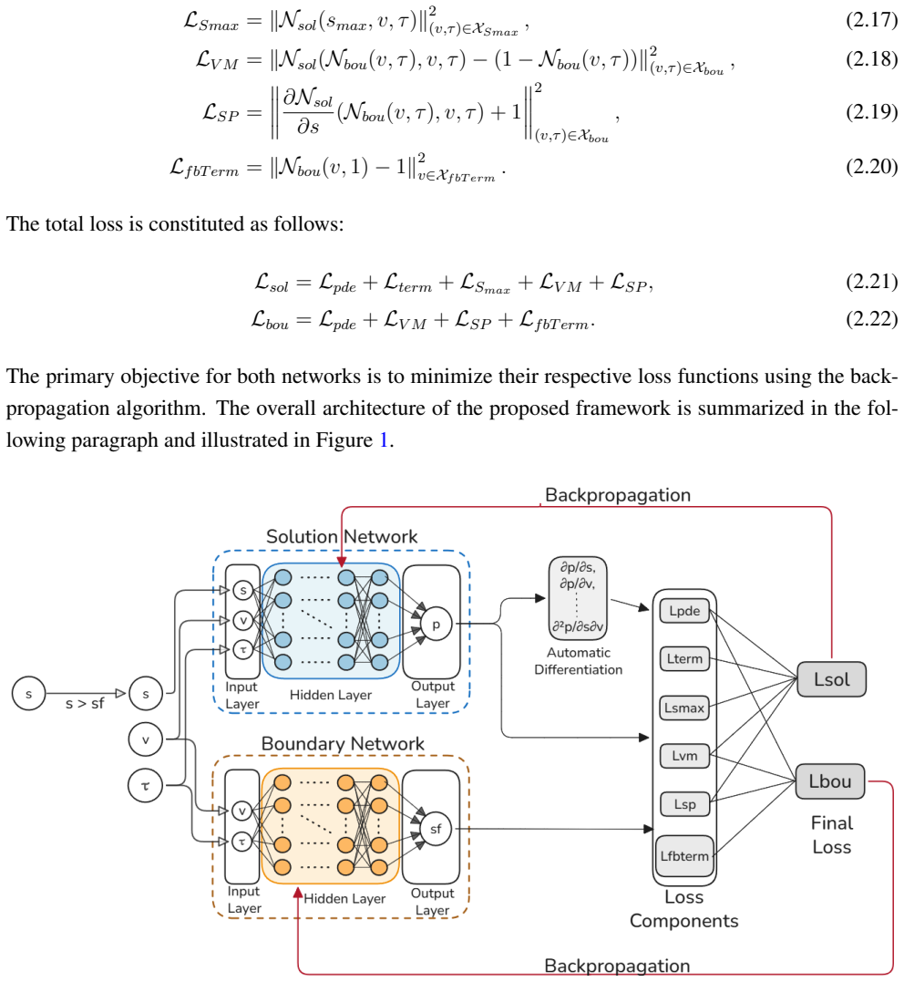
Coupled physics-informed neural networks in which the price network and the boundary network are optimized jointly so that the PDE residual, terminal payoff, and free-boundary conditions are all enforced in the loss function.
If this is right
- The networks produce option prices and exercise boundaries that agree with established numerical references for typical American put contracts.
- After training, prices at any time and asset level can be obtained in milliseconds without re-solving a grid.
- Curriculum learning and adaptive resampling reduce the sensitivity of training compared with plain physics-informed optimization.
- The method supplies a mesh-free alternative to finite-difference or Monte Carlo schemes for stochastic-volatility American pricing.
- Rapid evaluation opens the door to repeated pricing inside larger risk or hedging calculations.
Where Pith is reading between the lines
- The same coupled-network structure could be reused for American options under other volatility dynamics such as SABR or rough-volatility models.
- Fast forward passes would allow real-time calculation of Greeks or portfolio sensitivities that include early-exercise effects.
- The networks could be placed inside an outer optimization loop to calibrate model parameters to observed American option quotes.
- The approach might transfer to other free-boundary problems in finance, such as optimal stopping decisions under stochastic control.
Load-bearing premise
The training procedure will converge reliably to the correct free-boundary solution rather than to unstable or inaccurate local minima.
What would settle it
For a standard set of Heston parameters, the network prices or boundaries deviate by more than a few basis points from reference values obtained by a fine-grid finite-difference solver or a binomial tree.
Figures


read the original abstract
In American options, the early exercise feature allows the option to be exercised at any time prior to expiration. However, this flexibility introduces a challenge: the pricing model must value the option while simultaneously determining an unknown, time-varying exercise boundary. The Heston model is one of the most popular ways to model real market behavior because it allows volatility to change over time. However, unlike European options, there is no closed-form solution for American options under the Heston model, so we have to use numerical methods. In this paper, we propose a novel approach to solving the stochastic Heston partial differential equation for American options, using coupled physics-informed neural networks (PINNs) to predict both the option price and the free boundary, while employing curriculum learning and adaptive resampling to stabilize model training. Our work builds on recent deep learning methods but introduces a more effective training strategy to address the limitations of these approaches. The numerical results demonstrate the effectiveness of the proposed learning framework, providing a robust and efficient alternative to pricing American options, enabling rapid inference and accurate estimation under stochastic volatility.
Editorial analysis
A structured set of objections, weighed in public.
Referee Report
Summary. The paper proposes a coupled physics-informed neural network (PINN) framework, augmented with curriculum learning and adaptive resampling, to solve the free-boundary PDE arising from American option pricing under the Heston stochastic volatility model. The method simultaneously predicts the option price and the time-dependent exercise boundary, claiming to provide a robust, efficient alternative to traditional numerical methods with the advantage of rapid inference after training.
Significance. If the numerical results can be shown to match or exceed the accuracy of established methods (e.g., finite-difference schemes or Monte Carlo with regression) while delivering fast inference, the work would add a useful data-driven tool for pricing American options with stochastic volatility. The curriculum-learning and adaptive-resampling strategies address known training difficulties in free-boundary PINNs and therefore represent a plausible incremental advance, but the significance hinges on quantitative validation that is currently absent.
major comments (3)
- [Abstract and §4] Abstract and §4 (Numerical Results): the claim that 'the numerical results demonstrate the effectiveness of the proposed learning framework' is unsupported because no quantitative metrics (L² or L^∞ errors, convergence rates, or direct comparisons against finite-difference or other PINN baselines) are reported, nor is any detail given on how the free-boundary complementarity condition is enforced in the loss.
- [§3] §3 (Methodology): the coupled-PINN loss formulation is described only at a high level; the precise weighting of the PDE residual, boundary losses, and free-boundary penalty terms, together with the mechanism that couples the price and boundary networks, must be stated explicitly so that readers can verify that the American early-exercise condition is correctly imposed.
- [§4 and §5] §4 and §5: no sensitivity study or ablation on hyper-parameter choices (network depth/width, loss weights, curriculum schedule, resampling frequency) is provided, leaving the weakest assumption—that the method converges reliably without significant initialization or hyper-parameter dependence—unexamined.
minor comments (2)
- [§2] Notation for the Heston parameters (κ, θ, σ, ρ) and the free-boundary function B(t) should be introduced once in §2 and used consistently thereafter.
- [§4] A brief comparison table listing training time, inference time, and error against at least one standard benchmark (e.g., the Heston finite-difference solver) would greatly improve readability of the results section.
Simulated Author's Rebuttal
We thank the referee for the constructive and detailed comments. We address each major point below and will revise the manuscript accordingly to strengthen the presentation of results and methodology.
read point-by-point responses
-
Referee: [Abstract and §4] Abstract and §4 (Numerical Results): the claim that 'the numerical results demonstrate the effectiveness of the proposed learning framework' is unsupported because no quantitative metrics (L² or L^∞ errors, convergence rates, or direct comparisons against finite-difference or other PINN baselines) are reported, nor is any detail given on how the free-boundary complementarity condition is enforced in the loss.
Authors: We agree that the current manuscript would benefit from explicit quantitative validation. In the revised version we will add tables reporting L² and L^∞ errors for both the option price and the free boundary, computed against a high-resolution finite-difference reference solution. We will also include convergence plots with respect to training iterations and network capacity. Regarding the complementarity condition, we will explicitly state that it is enforced by augmenting the loss with a penalty term ∫ max(V - payoff, 0) dx dt over the continuation region, whose weight is chosen to balance the PDE residual. revision: yes
-
Referee: [§3] §3 (Methodology): the coupled-PINN loss formulation is described only at a high level; the precise weighting of the PDE residual, boundary losses, and free-boundary penalty terms, together with the mechanism that couples the price and boundary networks, must be stated explicitly so that readers can verify that the American early-exercise condition is correctly imposed.
Authors: We will expand Section 3 with the exact loss expression L = λ_PDE L_PDE + λ_BC L_BC + λ_FB L_FB + λ_comp L_comp, providing the numerical values used for each λ. The coupling mechanism will be described as follows: the boundary network outputs the time-dependent exercise boundary b(t), which is then used to partition the spatial domain for the price network; the price network is trained only in the continuation region while the complementarity penalty is applied globally. This formulation ensures the early-exercise condition is imposed both by domain restriction and by the penalty term. revision: yes
-
Referee: [§4 and §5] §4 and §5: no sensitivity study or ablation on hyper-parameter choices (network depth/width, loss weights, curriculum schedule, resampling frequency) is provided, leaving the weakest assumption—that the method converges reliably without significant initialization or hyper-parameter dependence—unexamined.
Authors: We acknowledge the absence of systematic hyper-parameter studies. In the revised manuscript we will add a dedicated subsection containing ablation experiments that vary network depth and width, the relative loss weights, the number of curriculum stages, and the frequency of adaptive resampling. For each variation we will report both final accuracy and training stability metrics, thereby addressing concerns about initialization and hyper-parameter sensitivity. revision: yes
Circularity Check
No circularity: standard PINN residual minimization for free-boundary PDE
full rationale
The paper applies coupled PINNs to minimize the Heston PDE residual plus boundary and free-boundary losses, augmented by curriculum learning and adaptive resampling. This is a direct numerical solver construction with no self-definitional loops, no fitted parameters renamed as predictions, and no load-bearing self-citations that reduce the central claim to prior author work. Numerical results are presented as empirical validation of the training strategy rather than a closed derivation that collapses to its inputs.
Axiom & Free-Parameter Ledger
free parameters (1)
- PINN hyperparameters (network depth, width, loss weights)
axioms (1)
- domain assumption The Heston stochastic volatility model PDE with free boundary condition for American options
Lean theorems connected to this paper
-
IndisputableMonolith/Cost/FunctionalEquation.leanwashburn_uniqueness_aczel unclearcoupled physics-informed neural networks (PINNs) to predict both the option price and the free boundary, while employing curriculum learning and adaptive resampling
-
IndisputableMonolith/Foundation/AlexanderDuality.leanalexander_duality_circle_linking unclearHeston PDE ... free-boundary problem
Reference graph
Works this paper leans on
-
[1]
and Guha, S
Aitsahlia, F., Goswami, M. and Guha, S. (2010). American option pricing under stochastic volatil- ity: an efficient numerical approach.Computational Management Science7, 171-187
2010
-
[2]
and Toivanen, J
Balajewicz, M. and Toivanen, J. (2016). Reduced Order Models for Pricing American Options under Stochastic V olatility and Jump-diffusion Models.Procedia Computer Science,80, 734-743
2016
-
[3]
and Scholes, M
Black, F. and Scholes, M. S. (1973). The pricing of options and corporate liabilities.Journal of Political Economy81(3), 637–654
1973
-
[4]
Bolaky, B. S. K., Narsoo, J., Thakoor, N., Tangman, D. Y . and Bhuruth, M. (2025). Deep neural networks for the valuation of equity and real-estate index American options under models with stochastic volatility.China Finance Review International(ahead-of-print)
2025
-
[5]
H., Chiarella, C
Cheang, G. H., Chiarella, C. and Ziogas, A. (2011). The representation of American options prices under stochastic volatility and jump-diffusion dynamics.Quantitative Finance13(2), 241-253. 23
2011
-
[6]
and Muthuraman, K
Chockalingam, A. and Muthuraman, K. (2011). American Options Under Stochastic V olatility. Operations Research59(4), 793-809
2011
-
[7]
and Parrott, K
Clarke, N. and Parrott, K. (1999). Multigrid for American option pricing with stochastic volatility. Applied Mathematical Finance6(3), 177-195
1999
-
[8]
Gatta, F., Schiano, D. C. V ., Giampaolo, F., Piccialli, F. and Cuomo, S. (2023). Meshless methods for American option pricing through Physics-Informed Neural Networks.Engineering Analysis with Boundary Elements151, 68-82
2023
-
[9]
and Casas, P
Hainaut, D. and Casas, P. (2024). Option pricing in the Heston model with physics inspired neural networks.Annals of Finance20(3), 353-376
2024
-
[10]
and E, W
Han, J., Jentzen, A. and E, W. (2018). Solving High-Dimensional Partial Differential Equations Using Deep Learning.Proceedings of the National Academy of Sciences115(34), 8505-8510
2018
-
[11]
Hanson, F. B. and Yan, G. (2007). Finite difference methods for pricing American options with stochastic volatility and jump-diffusion.Proceedings of the 2007 American Control Conference, New York, NY , United States
2007
-
[12]
Gaussian Error Linear Units (GELUs)
Hendrycks, D. and Gimpel, K. (2023). Gaussian Error Linear Units (GELUs).arXiv preprint arXiv:1606.08415
work page internal anchor Pith review Pith/arXiv arXiv 2023
-
[13]
Heston, S. L. (1993). A closed-form solution for options with stochastic volatility with applica- tions to bond and currency options.The Review of Financial Studies6(2), 327–343
1993
-
[14]
and Tomas, M
Horvath, B., Muguruza, A. and Tomas, M. (2021). Deep Learning V olatility: A Deep Neural Net- work Perspective on Pricing and Calibration in (Rough) V olatility Models,Quantitative Finance, 21(8), 11-27
2021
-
[15]
M., Lo, A
Hutchinson, J. M., Lo, A. W. and Poggio, T. (1994). A Nonparametric Approach to Pricing and Hedging Derivative Securities Via Learning Networks,The Journal of Finance,49(3), 851-889
1994
-
[16]
and Toivanen, J
Ikonen, S. and Toivanen, J. (2009). Operator splitting methods for pricing American options under stochastic volatility.Numerische Mathematik113(2), 299-324
2009
-
[17]
Koffi, R. S. and Tambue, A. (2021). A Fitted L-Multi-Point Flux Approximation Method for Pricing Options,Computational Economics60, 633–663
2021
-
[18]
Krishnapriyan, S., Gholami, A., Zhe, S., Kirby, R. and Mahoney, M. W. (2021). Characterizing Possible Failure Modes in Physics-Informed Neural Networks.arXiv preprint arXiv:2101.10382. 24
-
[19]
Longstaff, F. A. and Schwartz, E. S. (2001). Valuing American options by simulation: a simple least-squares approach.The Review of Financial Studies14(1), 113-147
2001
-
[20]
Louskos, I. (2021). Physics-Informed Neural Networks for Option Pricing.Undergraduate Thesis, Dartmouth College
2021
-
[21]
and Dai, W
Nwankwo, C., Ware, T. and Dai, W. (2025). Ensemble deep neural network method for solving free boundary American style stochastic volatility models.Applied Intelligence55(2), 158
2025
-
[22]
and Viktor, H
Olorunnimbe, K. and Viktor, H. (2023). Deep learning in the stock market—a systematic survey of practice, backtesting, and applications,Artificial Intelligence Review,46, 2057–2109
2023
-
[23]
and Karniadakis, G
Raissi, M., Perdikaris, P. and Karniadakis, G. E. (2019). Physics-Informed Neural Networks: A Deep Learning Framework for Solving Forward and Inverse Problems Involving Nonlinear Partial Differential Equations.Journal of Computational Physics378, 686-707
2019
-
[24]
Rouah, F. D. (2013). The Heston Model and Its Extensions in Matlab and C#.Wiley Finance
2013
-
[25]
and Spiliopoulos, K
Sirignano, J. and Spiliopoulos, K. (2018). DGM: A Deep Learning Algorithm for Solving Partial Differential Equations.Journal of Computational Physics375, 1339-1364
2018
-
[26]
Thakoor, N., Tangman, D. Y . and Bhuruth, M. (2018). RBF-FD schemes for option valuation under models with price-dependent and stochastic volatility.Engineering Analysis with Boundary Elements92, 207-217
2018
-
[27]
Zhu, S. P. and Chen, W. T. (2011). A predictor–corrector scheme based on the ADI method for pricing American puts with stochastic volatility.Computers & Mathematics with Applications 62(1), 1-26
2011
-
[28]
and Chiarella, C
Ziogas, A. and Chiarella, C. (2005). Pricing American Options under Stochastic V olatility.Com- puting in Economics and Finance 2005, Society for Computational Economics77
2005
-
[29]
Zvan, R., Forsyth, P. A. and Vetzal, K. R. (1998). Penalty methods for American options with stochastic volatility.Journal of Computational and Applied Mathematics91(2), 199-218. 25
1998
discussion (0)
Sign in with ORCID, Apple, or X to comment. Anyone can read and Pith papers without signing in.