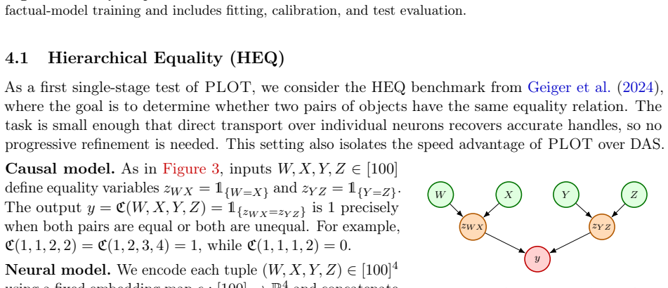
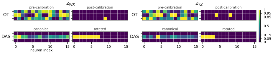
arxiv: 2605.06979 · v1 · submitted 2026-05-07 · 💻 cs.LG · cs.AI· stat.ML

Recognition: 2 theorem links

· Lean Theorem

PLOT: Progressive Localization via Optimal Transport in Neural Causal Abstraction

Arya Datla, Jonathn Chang, Ziv Goldfeld

Pith reviewed 2026-05-11 00:57 UTC · model grok-4.3

classification 💻 cs.LG cs.AIstat.ML

keywords causal abstractionoptimal transportmechanistic interpretabilityneural networksintervention analysislocalization

0 comments

The pith

Optimal transport couplings between intervention effects localize causal variables in neural networks.

A machine-rendered reading of the paper's core claim, the machinery that carries it, and where it could break.

The paper introduces PLOT to locate the parts of a neural network that realize specific causal variables from a high-level model. It does this by solving an optimal transport problem that pairs the output changes caused by intervening on abstract variables with the changes caused by intervening on candidate neural sites. The resulting coupling gives a soft correspondence that can be turned into intervention handles, applied in stages from large regions to small groups of neurons, and used to initialize faster searches. This matters because exhaustive search over neural sites becomes too slow for big models, while transport matching stays fast and accurate.

Core claim

PLOT fits an optimal transport coupling between abstract variables and candidate neural sites based on the geometry of their intervention output effects, yielding a global soft correspondence that identifies the neural handles for causal variables and supports progressive refinement or guidance of other methods.

What carries the argument

Optimal transport coupling over intervention output geometries, which establishes soft alignments between abstract causal variables and neural sites.

If this is right

In simple cases a single coupling over neurons gives accurate handles quickly.
When guiding DAS, it reaches similar accuracy with much less computation.
Progressive localization from tokens or layers down to finer spans makes the approach work on larger networks.
It offers a scalable way to perform causal abstraction analysis.

Where Pith is reading between the lines

These are editorial extensions of the paper, not claims the author makes directly.

The same transport idea could apply to aligning other kinds of high-level descriptions with network internals beyond causal models.
If it works reliably, researchers might use it to check proposed causal structures against actual network behavior more routinely.
It might inspire hybrid methods that combine transport with other alignment techniques for even better efficiency.

Load-bearing premise

That the geometry of output effects from abstract and neural interventions admits a meaningful optimal transport coupling corresponding to true causal variable alignments.

What would settle it

A test case with known correct neural sites where the transport coupling selects different sites and intervening there does not match the abstract model's counterfactual predictions.

Figures

Figures reproduced from arXiv: 2605.06979 by Arya Datla, Jonathn Chang, Ziv Goldfeld.

**Figure 1.** Figure 1: PLOT as a progressive localization engine. The diagram follows one high-level variable, Z2 in red, though OT localization is performed jointly over all high-level variables and candidate neural sites. PLOT first localizes coarse sites such as tokens/layers, then refines within them to coordinates or PCA spans. The resulting signal can be calibrated into a direct handle or used to guide DAS. discovering whe… view at source ↗

**Figure 2.** Figure 2: Optimal transport geometry & coupling. OT compares two probability distributions by the minimum cost of moving mass from one to the other. Given µ ∈ P(X ), ν ∈ P(Y), and a cost function c : X × Y → R, the Kantorovich OT problem is (Villani, 2003; Peyré and Cuturi, 2019) OTc(µ, ν) := inf π∈Π(µ,ν) Z c(x, y) dπ(x, y), where Π(µ, ν) := {π ∈ P(X × Y) : π(· × Y) = µ, π(X × ·) = ν} is the set of all couplings be… view at source ↗

**Figure 4.** Figure 4: HEQ comparison over 10 seeds. Values are mean ± standard deviation. Runtime excludes factual-model training and includes fitting, calibration, and test evaluation. 4.1 Hierarchical Equality (HEQ) As a first single-stage test of PLOT, we consider the HEQ benchmark from Geiger et al. (2024), where the goal is to determine whether two pairs of objects have the same equality relation. The task is small enough … view at source ↗

**Figure 3.** Figure 3: Causal model for HEQ. Causal model. As in [PITH_FULL_IMAGE:figures/full_fig_p007_3.png] view at source ↗

**Figure 5.** Figure 5: HEQ site-level intervention handles learned by OT (before and after calibration) and DAS (in the canonical and rotated basis). The two high-level variables are shown side by side. accurate, with average exact score 0.995 compared to 0.991 for PLOT. The larger difference is computational: PLOT takes 4.4 seconds on average, while DAS takes 131 seconds, making it roughly 30× slower end-to-end. Runtime include… view at source ↗

**Figure 6.** Figure 6: Causal model for 4-bit ripple-carry addition. Causal model. We consider 4-bit binary addition with inputs A3A2A1A0 and B3B2B1B0, as shown in [PITH_FULL_IMAGE:figures/full_fig_p008_6.png] view at source ↗

**Figure 7.** Figure 7: Binary-addition comparison over 10 seeds. Values are mean ± standard deviation. Accuracy is averaged over the internal carry variables C1, C2, C3, and runtime excludes backbone training [PITH_FULL_IMAGE:figures/full_fig_p009_7.png] view at source ↗

**Figure 8.** Figure 8: Binary-addition handles for d = 16. Rows show carries C1, C2, C3, while columns show postcalibration PLOT handles and PCA/DAS handles in their rotated bases. Two-stage PLOT and intervention handles. We use the same output effect pipeline as in HEQ, but with binary-addition-specific pair banks and recurrent candidate sites. Following the MIB Arithmetic benchmark (Mueller et al., 2025), we construct structu… view at source ↗

**Figure 9.** Figure 9: MCQA causal model, with abstract variables AP and AT. We next evaluate PLOT in the substantially larger setting of the MCQA benchmark from MIB (Mueller et al., 2025), where Gemma-2-2B answers natural-language multiplechoice prompts. The model reads a color fact and query, identifies the answer containing the queried color, and outputs its symbol. For example, given “The sky is blue. What color is the sk… view at source ↗

**Figure 10.** Figure 10: Additional HEQ diagnostics: sensitivity to entropic regularization and average learned intervention size. Effect of entropic regularization. We test sensitivity to the entropic regularization parameter ε in (1) by rerunning the HEQ PLOT pipeline on the same backbone and calibration protocol while varying only ε. As shown in Figure 10a, performance is stable once ε leaves the nearly unregularized regime. V… view at source ↗

read the original abstract

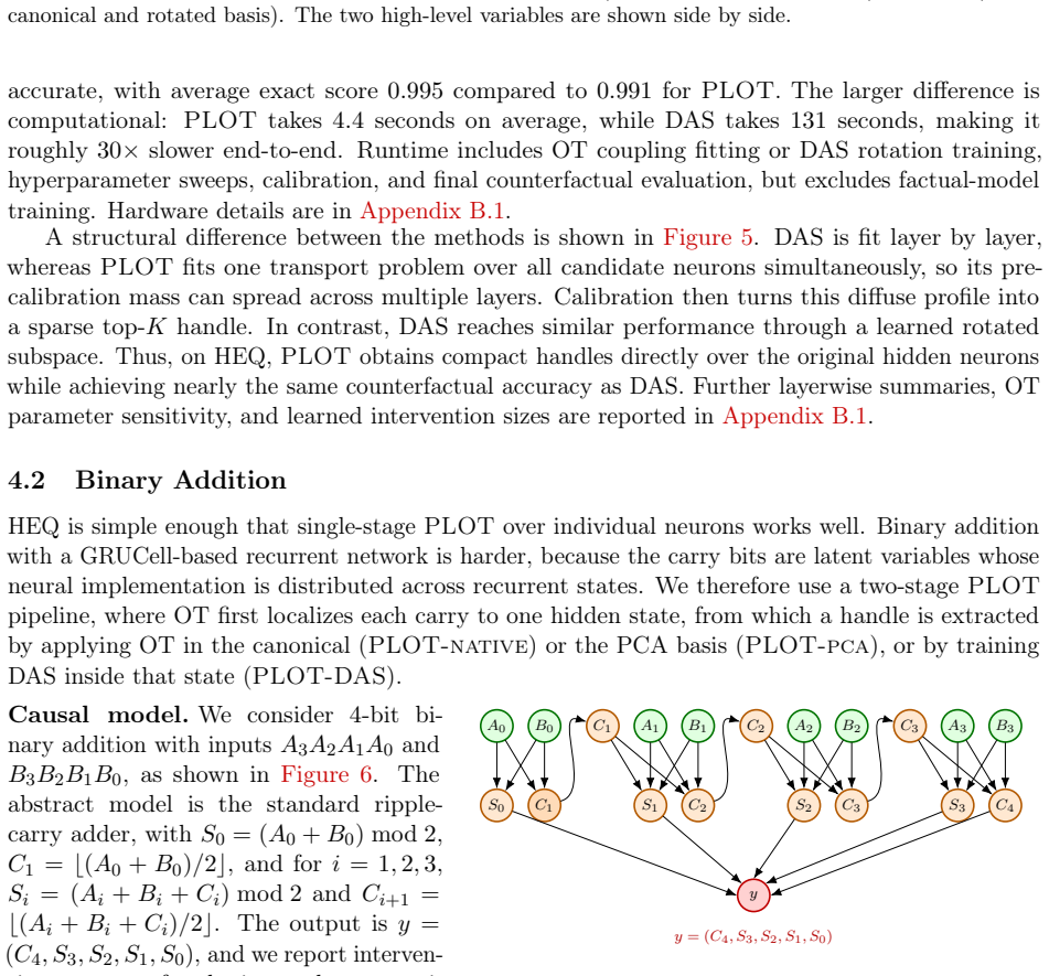
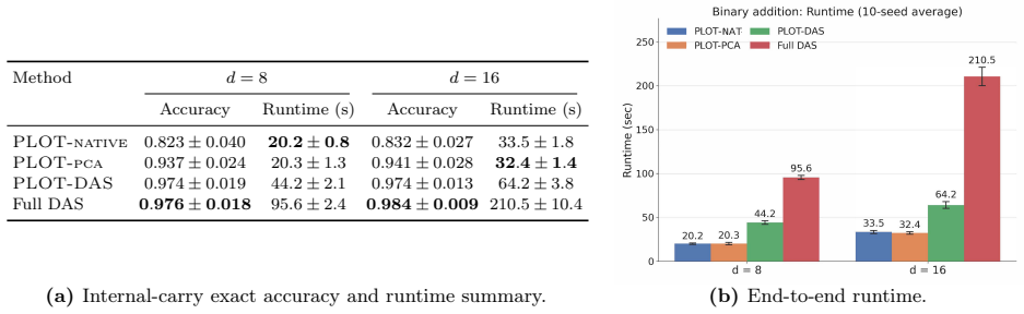
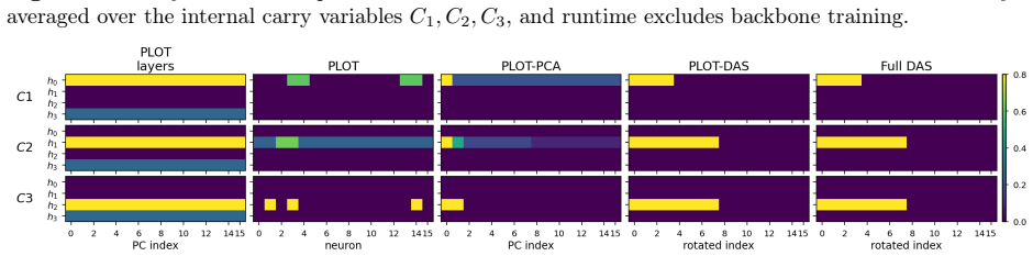
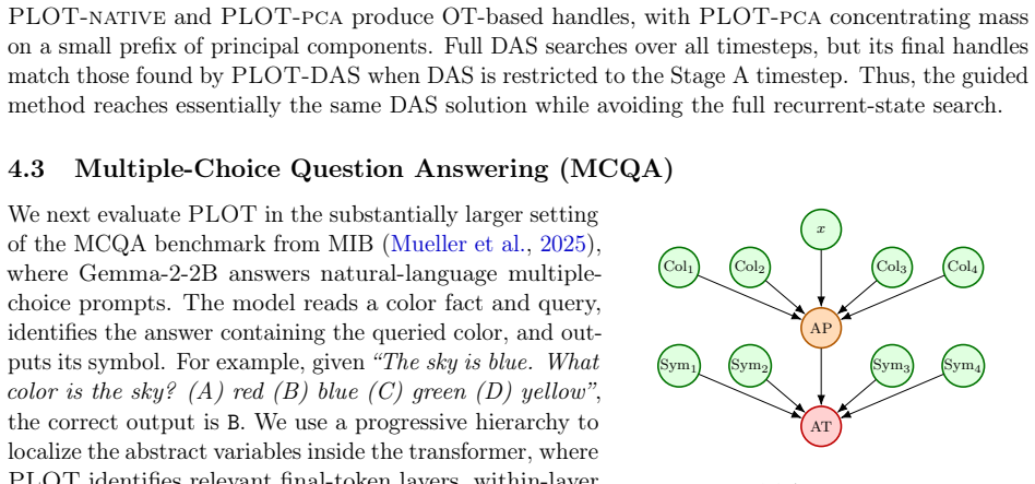
Causal abstraction offers a principled framework for mechanistic interpretability, aligning a high-level causal model with the low-level computation realized by a neural network through counterfactual intervention analysis. Existing methods such as distributed alignment search (DAS) learn expressive subspace interventions, but the relevant neural site is unknown a priori, so finding a handle requires a computationally burdensome search over candidate sites. We introduce PLOT (Progressive Localization via Optimal Transport), a transport-based framework that localizes causal variables from the output effect geometry of abstract and neural interventions. PLOT fits an optimal transport coupling between abstract variables and candidate neural sites, yielding a global soft correspondence that can be calibrated into intervention handles. In simple settings, a single coupling over individual neurons suffices. In larger models, PLOT is applied progressively, moving from coarse sites such as tokens, timesteps, or layers to finer supports such as coordinate groups or PCA spans, and optionally guiding DAS based on the localized signal. Across experiments of increasing complexity, transport-only PLOT handles are exceedingly fast and competitive on accuracy, while PLOT-guided DAS reaches DAS-level accuracy at a fraction of full DAS runtime, providing an efficient localization engine for causal abstraction research at scale.

Editorial analysis

A structured set of objections, weighed in public.

Desk editor's note, referee report, simulated authors' rebuttal, and a circularity audit. Tearing a paper down is the easy half of reading it; the pith above is the substance, this is the friction.

Desk Editor's Note private letter to a colleague

PLOT speeds up causal site localization in neural nets with progressive optimal transport on intervention effects, but risks spurious matches when those effects overlap across sites.

read the letter

PLOT uses optimal transport to match abstract causal variables to neural sites by comparing the geometry of output changes under interventions. It starts at coarse scales like layers or tokens and refines to finer groups or subspaces, then can feed the result into DAS for tighter handles. This cuts the search burden that full DAS faces when the right site is unknown ahead of time. The experiments on tasks of growing complexity show transport-only versions running fast with accuracy close to baselines, and the guided DAS version hitting similar performance in far less time. That practical efficiency is the clearest gain over prior search-heavy methods. The progressive schedule and the direct use of effect distributions for the coupling are the main technical moves that set it apart from standard DAS-style approaches. The paper reports solid runtime and accuracy numbers across those tests, which gives the claims some grounding. The main soft spot is the assumption that minimal-cost transport on effect vectors will recover the true causal correspondence. When multiple neural sites produce similar output perturbations, the coupling can align to the wrong location, and the coarse-to-fine steps may reinforce that error before finer checks can correct it. The abstract does not clarify whether success is scored by strict interchange equivalence or by looser effect matching, so it is hard to tell how often this happens in the reported runs. If the full experiments include controlled cases with overlapping effects, that would strengthen the result; otherwise the method needs more stress-testing on distributed representations. This work is aimed at interpretability researchers scaling causal abstraction to larger models where exhaustive search becomes impractical. Readers already using DAS or similar tools will see immediate value in the localization step even if they later add safeguards. It deserves a serious referee because it targets a real computational bottleneck with a concrete new technique and backs the speed claims with experiments. I would send it for review and ask specifically for checks on alignment accuracy under ambiguous effect geometries.

Referee Report

2 major / 2 minor

Summary. The manuscript introduces PLOT (Progressive Localization via Optimal Transport), a framework for localizing causal variables in neural networks by fitting optimal transport couplings between abstract variables and candidate neural sites based on the geometry of their intervention effects. It describes a progressive coarse-to-fine application from tokens/layers to finer supports and optional guidance for DAS, reporting that transport-only PLOT is fast and competitive in accuracy while PLOT-guided DAS achieves DAS-level performance at reduced runtime across experiments of increasing complexity.

Significance. If the OT-based couplings reliably recover true causal alignments rather than spurious effect matches, PLOT could provide a scalable localization engine that reduces the search burden in causal abstraction methods, enabling mechanistic interpretability at larger scales. The progressive schedule and DAS integration are practical strengths, but significance hinges on validation that effect-geometry transport corresponds to interchange-intervention equivalence.

major comments (2)

[Section 4] Section 4 (Experiments): the reported competitive accuracy on experiments of increasing complexity does not specify whether the metric is strict interchange-intervention equivalence (IIE) with the high-level model or a proxy based solely on output-effect matching. This distinction is load-bearing for the central claim, as the OT coupling is constructed precisely to minimize effect-geometry distance and could succeed on proxies without ensuring causal fidelity when multiple sites induce similar perturbations.
[Section 3.2] Section 3.2 (Progressive Localization): the coarse-to-fine schedule is presented without analysis or safeguards against early incorrect soft alignments propagating to finer supports (e.g., coordinate groups or PCA spans). If an initial token- or layer-level coupling selects a spurious site due to similar intervention effects, the subsequent refinement cannot recover the true causal variable.

minor comments (2)

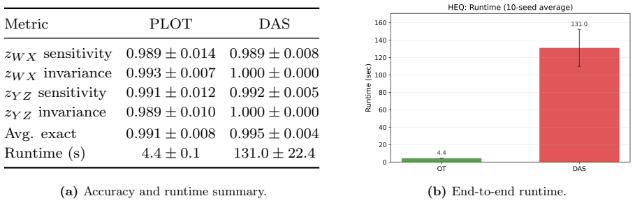
[Abstract] Abstract: the claim that 'transport-only PLOT handles are exceedingly fast' lacks quantitative runtime tables or speedup factors relative to exhaustive DAS search, reducing clarity on the efficiency contribution.
[Method] Notation throughout: the cost function used for the OT plan (distance between effect vectors or distributions) is not explicitly defined with an equation, making it difficult to assess uniqueness or robustness to distributed representations.

Simulated Author's Rebuttal

2 responses · 0 unresolved

We thank the referee for the careful reading and insightful comments, which help clarify the presentation of our results and the robustness of the progressive localization procedure. We address each major comment below and indicate the corresponding revisions.

read point-by-point responses

Referee: [Section 4] Section 4 (Experiments): the reported competitive accuracy on experiments of increasing complexity does not specify whether the metric is strict interchange-intervention equivalence (IIE) with the high-level model or a proxy based solely on output-effect matching. This distinction is load-bearing for the central claim, as the OT coupling is constructed precisely to minimize effect-geometry distance and could succeed on proxies without ensuring causal fidelity when multiple sites induce similar perturbations.

Authors: We agree that this distinction is important. The accuracy numbers reported in Section 4 are computed using the standard interchange-intervention accuracy metric from the causal abstraction literature (i.e., the fraction of test inputs on which the low-level model with the learned intervention matches the high-level model under interchange interventions). This is the same metric used to evaluate DAS and is directly tied to IIE rather than a pure output-effect proxy. Nevertheless, to make the evaluation fully transparent and to address the referee’s concern about possible spurious effect matches, we will add an explicit statement of the metric in Section 4, include a short derivation showing why the OT objective is consistent with IIE under the linear-intervention assumption used in our experiments, and report an additional column of strict IIE success rates (exact match on all counterfactuals) for the main tables. These changes will appear in the revised manuscript. revision: yes
Referee: [Section 3.2] Section 3.2 (Progressive Localization): the coarse-to-fine schedule is presented without analysis or safeguards against early incorrect soft alignments propagating to finer supports (e.g., coordinate groups or PCA spans). If an initial token- or layer-level coupling selects a spurious site due to similar intervention effects, the subsequent refinement cannot recover the true causal variable.

Authors: This is a valid concern. The current manuscript presents the progressive schedule as a practical heuristic without a formal analysis of error propagation. In practice, the coarse-stage couplings are stable because intervention-effect geometries are more separable at the token/layer level, and the soft OT plan retains probability mass on multiple candidates that are then refined. To strengthen the paper, we will (i) add a paragraph in Section 3.2 discussing the conditions under which early-stage errors are unlikely (distinct effect geometries at coarse scales), (ii) include a small ablation that measures alignment stability across stages on the synthetic tasks, and (iii) describe an optional safeguard—retaining the top-k soft assignments from the coarse stage for parallel refinement at the fine stage. These additions will be incorporated in the revision. revision: yes

Circularity Check

0 steps flagged

No significant circularity in derivation chain

full rationale

The paper defines PLOT as a new transport-based localization procedure that computes an optimal transport coupling on intervention effect geometries and optionally guides DAS. This is a constructive definition of a method rather than a claim that reduces by construction to its inputs. No load-bearing steps invoke self-citations, fitted parameters renamed as predictions, or uniqueness theorems from prior author work. Empirical accuracy claims are presented as experimental outcomes on held-out or increasing-complexity tasks, not as tautological consequences of the fitting procedure itself. The derivation chain therefore remains self-contained against external benchmarks.

Axiom & Free-Parameter Ledger

0 free parameters · 1 axioms · 0 invented entities

Abstract provides insufficient detail to enumerate specific free parameters or axioms; the core assumption is that OT couplings on intervention geometries align with causal variables.

axioms (1)

domain assumption Intervention effect geometries can be meaningfully coupled via optimal transport to recover causal variable locations
Central to the PLOT framework as stated in the abstract

pith-pipeline@v0.9.0 · 5513 in / 1110 out tokens · 43712 ms · 2026-05-11T00:57:10.495200+00:00 · methodology

discussion (0)

Lean theorems connected to this paper

Citations machine-checked in the Pith Canon. Every link opens the source theorem in the public Lean library.

IndisputableMonolith/Cost/FunctionalEquation.lean washburn_uniqueness_aczel unclear
PLOT fits an optimal transport coupling between abstract variables and candidate neural sites, yielding a global soft correspondence that can be calibrated into intervention handles.
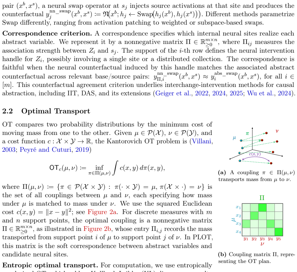
IndisputableMonolith/Foundation/BranchSelection.lean branch_selection unclear
We use the squared Euclidean cost c(x, y) = ∥x−y∥²

Reference graph

Works this paper leans on

20 extracted references · 16 canonical work pages · 5 internal anchors

[1]

URL https://doi.org/10.1016/j.spa.2019.08.009

doi: 10.1016/j.spa.2019.08.009. URL https://doi.org/10.1016/j.spa.2019.08.009. T. Bricken, A. Templeton, J. Batson, B. Chen, A. Jermyn, T. Conerly, N. Turner, C. Anil, C. Denison, A. Askell, R. Lasenby, Y. Wu, S. Kravec, N. Schiefer, T. Maxwell, N. Joseph, Z. Hatfield-Dodds, A. Tamkin, K. Nguyen, B. McLean, J. E. Burke, T. Hume, S. Carter, T. Henighan, an...

work page doi:10.1016/j.spa.2019.08.009 2019
[2]

Maheep Chaudhary and Atticus Geiger

URLhttps://transformer-circuits.pub/2023/monosemantic-features/ index.html. Maheep Chaudhary and Atticus Geiger. Evaluating open-source sparse autoencoders on disentangling factual knowledge in GPT-2 small.CoRR, abs/2409.04478,

work page arXiv 2023
[3]

Maheep Chaudhary and Atticus Geiger

doi: 10.48550/arXiv.2409.04478. URLhttps://arxiv.org/abs/2409.04478. Patrick Cheridito and Stephan Eckstein. Optimal transport and Wasserstein distances for causal models.Bernoulli, 31(2):1351–1376,

work page doi:10.48550/arxiv.2409.04478
[4]

URLhttps://doi.org/10

doi: 10.3150/24-BEJ1773. URLhttps://doi.org/10. 3150/24-BEJ1773. Lénaïc Chizat, Gabriel Peyré, Bernhard Schmitzer, and François-Xavier Vialard. Scaling algorithms for unbalanced transport problems.Mathematics of Computation, 87(314):2563–2609,

work page doi:10.3150/24-bej1773
[5]

Sparse Autoencoders Find Highly Interpretable Features in Language Models

Hoagy Cunningham, Aidan Ewart, Logan Riggs Smith, Robert Huben, and Lee Sharkey. Sparse autoencoders find highly interpretable features in language models.CoRR, abs/2309.08600,

work page internal anchor Pith review Pith/arXiv arXiv
[6]

Sparse Autoencoders Find Highly Interpretable Features in Language Models

doi: 10.48550/arXiv.2309.08600. URLhttps://arxiv.org/abs/2309.08600. Marco Cuturi. Sinkhorn distances: Lightspeed computation of optimal transport. InAdvances in Neural Information Processing Systems, volume 26,

work page internal anchor Pith review Pith/arXiv arXiv doi:10.48550/arxiv.2309.08600
[7]

Gemma 2: Improving Open Language Models at a Practical Size

Gemma Team. Gemma 2: Improving open language models at a practical size.CoRR, abs/2408.00118,

work page internal anchor Pith review Pith/arXiv arXiv
[8]

Gemma 2: Improving Open Language Models at a Practical Size

doi: 10.48550/arXiv.2408.00118. URLhttps://arxiv.org/abs/2408.00118. Robert Huben, Hoagy Cunningham, Logan Riggs Smith, Aidan Ewart, and Lee Sharkey. Sparse autoencoders find highly interpretable features in language models. InThe Twelfth Interna- tional Conference on Learning Representations,

work page internal anchor Pith review Pith/arXiv arXiv doi:10.48550/arxiv.2408.00118
[10]

Adam: A Method for Stochastic Optimization

URLhttps://arxiv.org/abs/1412.6980. Rémi Lassalle. Causal transport plans and their Monge–Kantorovich problems.Stochastic Analysis and Applications, 36(3):452–484,

work page internal anchor Pith review Pith/arXiv arXiv
[11]

URLhttps://doi

doi: 10.1080/07362994.2017.1422747. URLhttps://doi. org/10.1080/07362994.2017.1422747. Samuel Marks and Max Tegmark. The geometry of truth: Emergent linear structure in large language model representations of true/false datasets. InFirst Conference on Language Modeling,

work page doi:10.1080/07362994.2017.1422747 2017
[12]

Interpretability analysis of arithmetic in-context learning in large language models

Gregory Polyakov, Christian Hepting, Carsten Eickhoff, and Seyed Ali Bahrainian. Interpretability analysis of arithmetic in-context learning in large language models. InProceedings of the 2025 Conference on Empirical Methods in Natural Language Processing, pages 1758–1777,

2025
[13]

URLhttps://aclanthology.org/2025.emnlp-main.92/

doi: 10.18653/v1/2025.emnlp-main.92. URLhttps://aclanthology.org/2025.emnlp-main.92/. Jiuding Sun, Jing Huang, Sidharth Baskaran, Karel D’Oosterlinck, Christopher Potts, Michael Sklar, and Atticus Geiger. HyperDAS: Towards automating mechanistic interpretability with hypernetworks.CoRR, abs/2503.10894,

work page doi:10.18653/v1/2025.emnlp-main.92 2025
[14]

Curt Tigges, Oskar John Hollinsworth, Atticus Geiger, and Neel Nanda

URLhttps://arxiv.org/abs/2503.10894. Curt Tigges, Oskar John Hollinsworth, Atticus Geiger, and Neel Nanda. Linear representations of sentiment in large language models.CoRR, abs/2310.15154,

work page arXiv
[15]

J., Geiger, A., and Nanda, N

doi: 10.48550/arXiv.2310.15154. URLhttps://arxiv.org/abs/2310.15154. Dor Tsur and Ziv Goldfeld. Neural entropic multi-marginal optimal transport and Gromov– Wasserstein alignment.CoRR, abs/2506.00573,

work page doi:10.48550/arxiv.2310.15154
[16]

URL https://arxiv.org/abs/2506.00573

doi: 10.48550/arXiv.2506.00573. URL https://arxiv.org/abs/2506.00573. 13 Cédric Villani.Topics in optimal transportation, volume 58 ofGraduate Studies in Mathematics. American Mathematical Society,

work page doi:10.48550/arxiv.2506.00573
[17]

URLhttps: //doi.org/10.1109/TIT.2026.3661439

doi: 10.1109/TIT.2026.3661439. URLhttps: //doi.org/10.1109/TIT.2026.3661439. Early access. Zhengxuan Wu, Atticus Geiger, Thomas Icard, Christopher Potts, and Noah D. Goodman. Inter- pretability at scale: Identifying causal mechanisms in Alpaca.CoRR, abs/2305.08809,

work page doi:10.1109/tit.2026.3661439 2026
[18]

14 Appendix A Additional Methodology Details We evaluate learned handles by interchange-intervention accuracy (Geiger et al., 2024)

URL https://arxiv.org/abs/2305.08809. 14 Appendix A Additional Methodology Details We evaluate learned handles by interchange-intervention accuracy (Geiger et al., 2024). For a handle associated withZ i, calibration accuracy is Lcal(Zi) := 1 Tcal TcalX t=1 1n ynn_swap Π,i (xb t ,xs t)=yabs_swap i (xb t ,xs t) o, with test accuracy defined analogously onDt...

work page arXiv 2024
[19]

Indeed, a method that learns no handle can score perfectly on invariance-heavy test sets, yielding high average accuracy while being weak on sensitivity

which mixed sensitive and invariant pairs, leading to test accuracies that are less interpretable. Indeed, a method that learns no handle can score perfectly on invariance-heavy test sets, yielding high average accuracy while being weak on sensitivity. Unless stated otherwise, main-text accuracies average over all2m sensitive and invariant test sets, two ...

2017
[20]

to obtainℓ AP andℓ AT 3:forZ∈ {AP,AT}do 4:fork∈ {32,64,96,128,256,512,768,1024,1536,2048,2304}do 5:Train a DAS rotation forZonD ft at layerℓ Z with subspace intervention sizek 6:Evaluate the rotation handle forZonD cal 7:end for 8:Evaluate the best calibrated rotation forZonD te 9:end for 10:End timer and reportPLOT-DASruntime Algorithm 10MCQAPLOT-native-...

2048
[21]

to obtainℓ AP,ℓ AT,R AP,R AT,H pca AP,H pca AT 3:forZ∈ {AP,AT}do 4:Extractb ⋆ andK ⋆ fromH pca Z 5:Set effective dimensione:=⌊rank(R Z)/b⋆⌋K ⋆ 6:fork∈ {0.5e,0.75e, e,1.5e,2.0e}do 7:Train a DAS rotation on top ofR Z forZonD ft (DAS rotation has sizeRk×rank(RZ )) 8:Evaluate the rotation forZonD cal 9:end for 10:Evaluate the best calibrated rotation forZonD ...

2048