Recognition: 1 theorem link
· Lean TheoremSystematic Comparison between Constrained Transport and Mixed Divergence Cleaning Methods for Astrophysical Magnetohydrodynamic Simulations
Pith reviewed 2026-05-11 03:10 UTC · model grok-4.3
The pith
Constrained transport outperforms Dedner's divergence cleaning in MHD simulations when magnetic fields localize or timesteps change suddenly.
A machine-rendered reading of the paper's core claim, the machinery that carries it, and where it could break.
Core claim
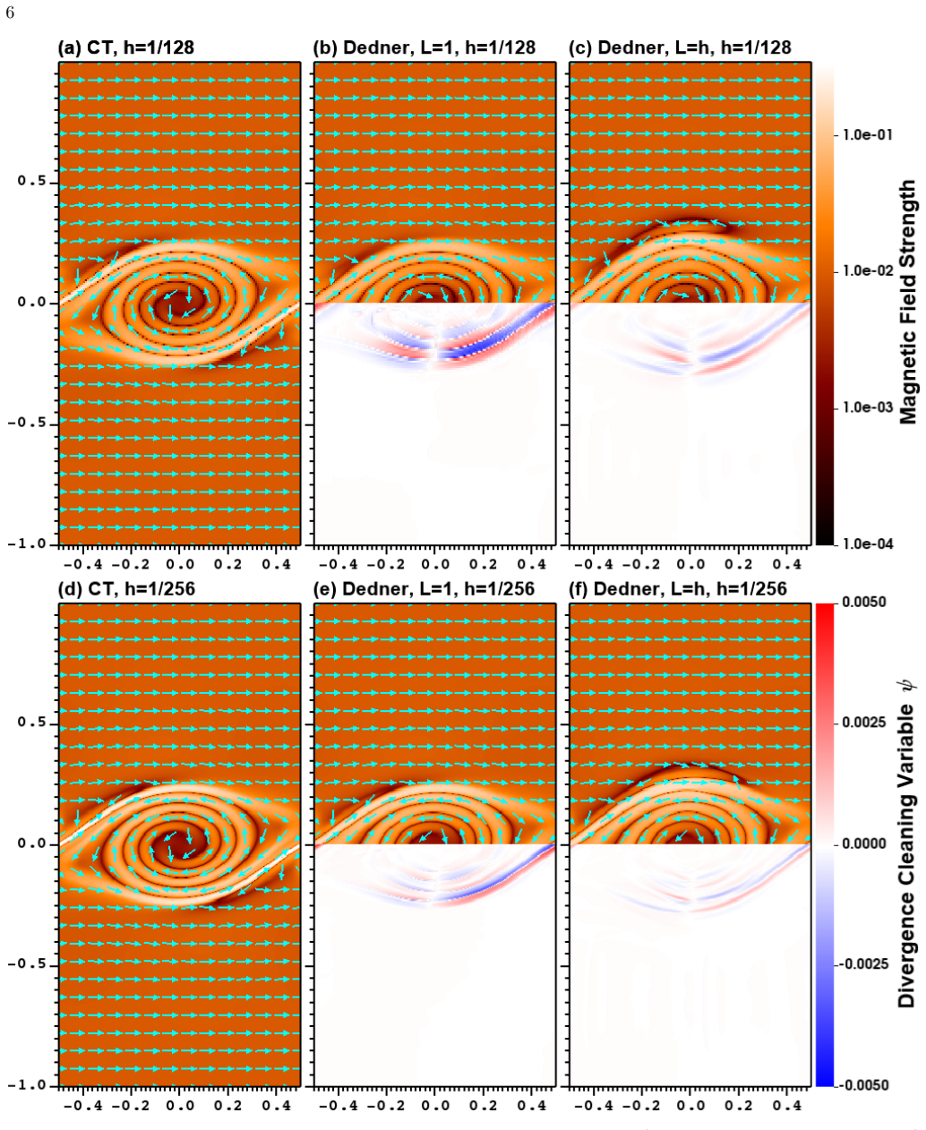
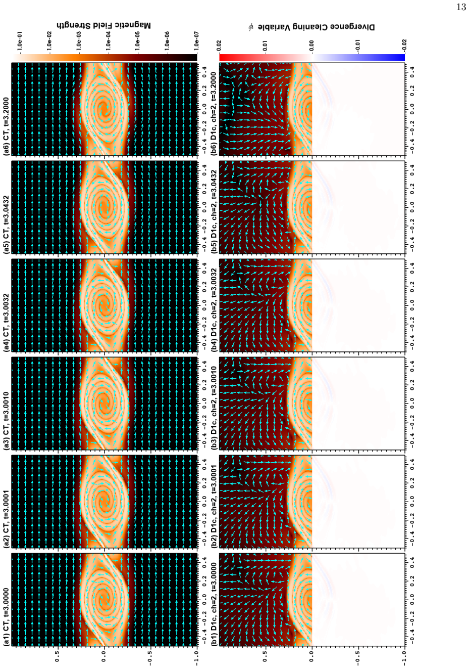
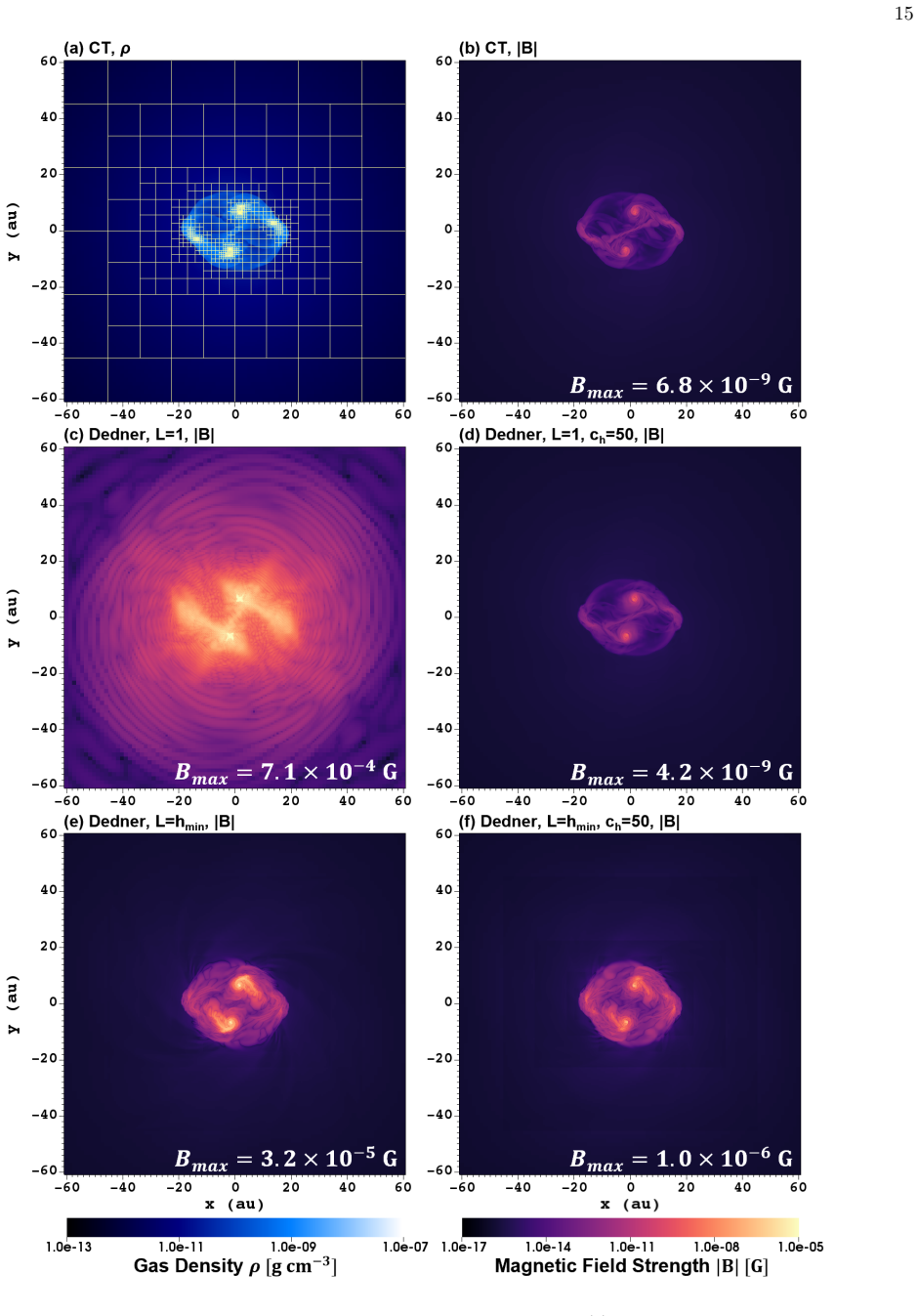
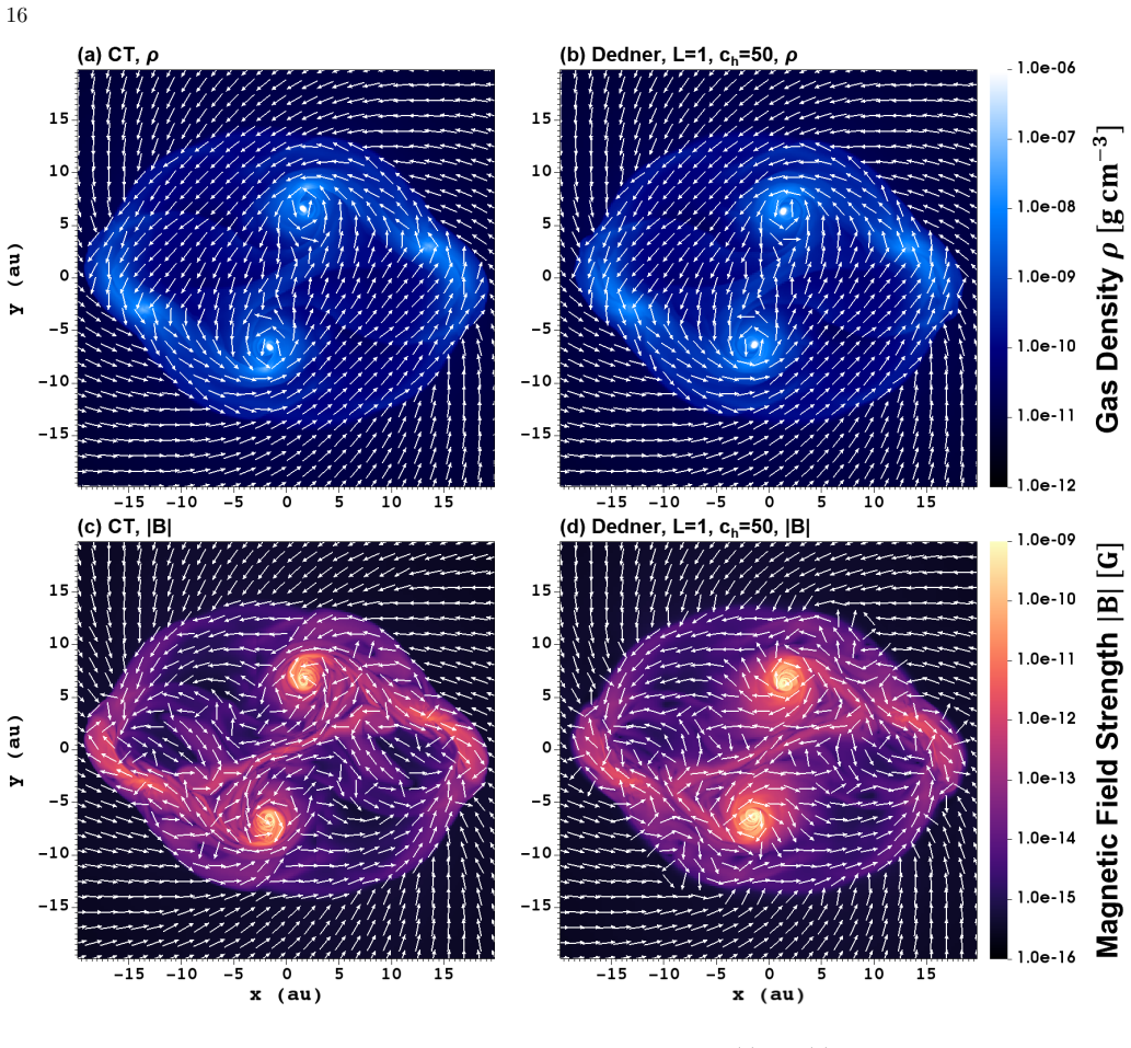
Numerical experiments show that the original Dedner's scheme becomes inaccurate when magnetic fields are strongly localized or when the timestep suddenly changes, while the constrained transport scheme maintains superior accuracy and reliability in enforcing the solenoidal constraint.
What carries the argument
Constrained transport on staggered grids versus Dedner's mixed divergence cleaning that introduces an additional variable to damp divergence errors in the MHD equations.
If this is right
- Previous claims of extremely rapid magnetic field growth in early-Universe star formation may require re-evaluation with constrained transport.
- Simulation codes using Dedner's scheme should consider adopting constrained transport or the proposed modifications for greater robustness.
- Divergence errors in localized-field regimes can contaminate physical interpretations unless the numerical method is chosen carefully.
- Modified Dedner's schemes may reduce but not eliminate the accuracy gap with constrained transport in variable-timestep runs.
Where Pith is reading between the lines
- Wider adoption of constrained transport could revise models of magnetic field amplification in collapsing astrophysical objects.
- Systematic tests in codes with adaptive timesteps would reveal whether the artifacts persist beyond the reported experiments.
- Other divergence-cleaning variants may share similar vulnerabilities to sudden field localization.
Load-bearing premise
The chosen idealized tests and practical applications represent the typical regimes where these methods are used in astrophysical MHD research.
What would settle it
A controlled MHD test with strongly localized magnetic fields and abrupt timestep changes in which Dedner's original scheme matches the accuracy of constrained transport without producing artifacts.
Figures


read the original abstract
Magnetohydrodynamic (MHD) simulations are indispensable research infrastructure in astrophysics today. In order to satisfy the solenoidal constraint of the MHD equations on discretized grids, modern simulation codes often employ either constrained transport (CT) with a staggered grid or divergence cleaning using an additional variable. We compare CT and Dedner's mixed divergence cleaning schemes systematically, and find that the divergence cleaning scheme can produce substantial artifacts in certain situations. Through numerical experiments including both idealized tests and practical applications, we show that the original implementation of Dedner's scheme becomes inaccurate when magnetic fields are strongly localized or when the timestep suddenly changes. We find that some previous results, such as the extremely rapid growth of magnetic fields during star formation in the early Universe, may be affected by the spurious behavior of the divergence cleaning scheme. We propose a few modifications to improve the robustness of the divergence cleaning method. Nevertheless, we find that the CT scheme is more accurate and reliable in many situations.
Editorial analysis
A structured set of objections, weighed in public.
Referee Report
Summary. The manuscript performs a systematic numerical comparison of constrained transport (CT) on staggered grids versus Dedner's mixed divergence cleaning for enforcing the solenoidal constraint in astrophysical MHD simulations. Through idealized test problems and practical applications, it identifies regimes where the original Dedner implementation produces substantial artifacts, specifically with strongly localized magnetic fields or abrupt timestep changes. The authors suggest that this behavior may have influenced certain prior results, including claims of extremely rapid magnetic field growth during early-Universe star formation, propose modifications to improve cleaning robustness, and conclude that CT is more accurate and reliable in many situations.
Significance. If the empirical findings hold, the work is significant for the astrophysical MHD community because it supplies concrete evidence of limitations in a widely adopted divergence-cleaning technique and offers practical guidance on method selection and fixes. The side-by-side testing across idealized and applied cases, together with the proposed modifications, directly aids reproducibility and reliability of future simulations.
major comments (2)
- Abstract and discussion: the assertion that 'some previous results, such as the extremely rapid growth of magnetic fields during star formation in the early Universe, may be affected by the spurious behavior of the divergence cleaning scheme' rests on extrapolation from the idealized and practical tests rather than a direct head-to-head re-simulation of the cited historical runs at equivalent resolution and initial conditions using CT within the same code base. This step is load-bearing for the strongest implication drawn from the comparison.
- Results section (practical applications): the manuscript does not report quantitative error norms, convergence rates, or direct side-by-side divergence-error time series for the practical astrophysical cases, making it difficult to assess the magnitude and statistical significance of the reported artifacts relative to CT.
Simulated Author's Rebuttal
We thank the referee for the constructive and detailed review, as well as for recognizing the potential significance of our findings for the astrophysical MHD community. We address the two major comments point by point below, indicating the revisions we plan to make.
read point-by-point responses
-
Referee: Abstract and discussion: the assertion that 'some previous results, such as the extremely rapid growth of magnetic fields during star formation in the early Universe, may be affected by the spurious behavior of the divergence cleaning scheme' rests on extrapolation from the idealized and practical tests rather than a direct head-to-head re-simulation of the cited historical runs at equivalent resolution and initial conditions using CT within the same code base. This step is load-bearing for the strongest implication drawn from the comparison.
Authors: We agree that a direct head-to-head re-simulation of the exact cited runs would constitute stronger evidence. Our current claim is based on the fact that the artifact-triggering conditions we identified (strongly localized magnetic fields and abrupt timestep changes) are present in the setups of the referenced early-Universe star-formation simulations that employed Dedner's cleaning. In the revised manuscript we will moderate the language in the abstract and discussion to describe this as a plausible concern that may warrant re-examination, rather than a definitive statement that prior results are affected. We will also add a short paragraph explaining the mapping between our test conditions and those in the cited literature. revision: partial
-
Referee: Results section (practical applications): the manuscript does not report quantitative error norms, convergence rates, or direct side-by-side divergence-error time series for the practical astrophysical cases, making it difficult to assess the magnitude and statistical significance of the reported artifacts relative to CT.
Authors: We accept this criticism. The revised manuscript will include quantitative L2 and L∞ norms of the divergence error for both CT and Dedner runs in the practical-application sections, together with time-series plots of the divergence error and, where the problem setup permits, a brief convergence study. These additions will allow readers to evaluate the size and significance of the observed differences. revision: yes
- Performing a direct re-simulation of the specific historical runs cited in the abstract and discussion at equivalent resolution and initial conditions using CT within the original code bases; such an exercise lies outside the scope of the present study and would require substantial additional code development and computational resources.
Circularity Check
No circularity: empirical side-by-side numerical comparison
full rationale
The paper performs direct numerical experiments comparing established CT and Dedner divergence-cleaning schemes on idealized tests plus practical applications. All claims (artifact identification, proposed modifications, and the inference that prior rapid B-field growth results may be affected) rest on those simulations rather than any derivation, fitted parameter, or self-referential prediction. No load-bearing self-citation, uniqueness theorem, or ansatz is invoked; the work is self-contained against external benchmarks.
Axiom & Free-Parameter Ledger
axioms (1)
- domain assumption The MHD equations require that the magnetic field remains divergence-free (div B = 0) on discretized grids.
Reference graph
Works this paper leans on
-
[1]
2021, PrincetonUniversity/athena: Athena++ v21.0, 21.0 Zenodo, doi: 10.5281/zenodo.4455880
Athena++ development team. 2021, PrincetonUniversity/athena: Athena++ v21.0, 21.0 Zenodo, doi: 10.5281/zenodo.4455880
-
[2]
Balsara, D. S. 2004, ApJS, 151, 149, doi: 10.1086/381377
-
[3]
Balsara, D. S., & Kim, J. 2004, ApJ, 602, 1079, doi: 10.1086/381051
-
[4]
Bonnor, W. B. 1956, MNRAS, 116, 351
work page 1956
-
[5]
Brackbill, J. U., & Barnes, D. C. 1980, Journal of Computational Physics, 35, 426, doi: 10.1016/0021-9991(80)90079-0
-
[6]
Bryan, G. L., Norman, M. L., O’Shea, B. W., et al. 2014, ApJS, 211, 19, doi: 10.1088/0067-0049/211/2/19
-
[7]
Jones, T. W. 2009, ApJS, 182, 519, doi: 10.1088/0067-0049/182/2/519
-
[8]
2002, Journal of Computational Physics, 175, 645, doi: 10.1006/jcph.2001.6961
Dedner, A., Kemm, F., Kr¨ oner, D., et al. 2002, Journal of Computational Physics, 175, 645, doi: 10.1006/jcph.2001.6961
-
[9]
1955, Zeitschrift fur Astrophysik, 36, 222
Ebert, R. 1955, Zeitschrift fur Astrophysik, 36, 222
work page 1955
-
[10]
Evans, C. R., & Hawley, J. F. 1988, ApJ, 332, 659, doi: 10.1086/166684
-
[11]
2006, A&A, 457, 371, doi: 10.1051/0004-6361:20065371
Fromang, S., Hennebelle, P., & Teyssier, R. 2006, A&A, 457, 371, doi: 10.1051/0004-6361:20065371
-
[12]
Fryxell, B., Olson, K., Ricker, P., et al. 2000, ApJS, 131, 273, doi: 10.1086/317361
-
[13]
Gardiner, T. A., & Stone, J. M. 2005, Journal of Computational Physics, 205, 509, doi: 10.1016/j.jcp.2004.11.016
-
[14]
Hawley, J. F., & Stone, J. M. 1995, Computer Physics Communications, 89, 127, doi: 10.1016/0010-4655(95)00190-Q
-
[15]
Hirano, S., & Machida, M. N. 2022, ApJL, 935, L16, doi: 10.3847/2041-8213/ac85e0
-
[16]
doi:10.1093/mnras/stv2180 , eprint =
Hopkins, P. F., & Raives, M. J. 2016, MNRAS, 455, 51, doi: 10.1093/mnras/stv2180
-
[17]
2013, in Astronomical Society of the Pacific Conference Series, Vol
Iwasaki, K., & Inutsuka, S.-I. 2013, in Astronomical Society of the Pacific Conference Series, Vol. 474, Numerical Modeling of Space Plasma Flows (ASTRONUM2012), ed. N. V. Pogorelov, E. Audit, & G. P. Zank, 239
work page 2013
-
[18]
2023, A&A, 673, A66, doi: 10.1051/0004-6361/202245359
Keppens, R., Popescu Braileanu, B., Zhou, Y., et al. 2023, A&A, 673, A66, doi: 10.1051/0004-6361/202245359
-
[19]
H., Li, Z.-Y., Chen, C.-Y., Tomida, K., & Zhao, B
Lam, K. H., Li, Z.-Y., Chen, C.-Y., Tomida, K., & Zhao, B. 2019, MNRAS, 489, 5326, doi: 10.1093/mnras/stz2436
-
[20]
Larson, R. B. 1969, MNRAS, 145, 271, doi: 10.1093/mnras/145.3.271
-
[21]
Latif, M. A., Schleicher, D. R. G., & Khochfar, S. 2023, ApJ, 945, 137, doi: 10.3847/1538-4357/acbcc2
-
[22]
Latif, M. A., Schleicher, D. R. G., & Schmidt, W. 2014, MNRAS, 440, 1551, doi: 10.1093/mnras/stu357
-
[23]
Machida, M. N., Hirano, S., & Basu, S. 2025, ApJ, 988, 6, doi: 10.3847/1538-4357/addc56
-
[24]
2016, A&A, 587, A32, doi: 10.1051/0004-6361/201526371
Masson, J., Chabrier, G., Hennebelle, P., Vaytet, N., & Commer¸ con, B. 2016, A&A, 587, A32, doi: 10.1051/0004-6361/201526371
-
[25]
2019, PASJ, 71, 83, doi: 10.1093/pasj/psz064
Matsumoto, Y., Asahina, Y., Kudoh, Y., et al. 2019, PASJ, 71, 83, doi: 10.1093/pasj/psz064
-
[26]
2024, A&A, 686, A253, doi: 10.1051/0004-6361/202348405
Mauxion, J., Lesur, G., & Maret, S. 2024, A&A, 686, A253, doi: 10.1051/0004-6361/202348405
-
[27]
Mayer, A. C., Zier, O., Naab, T., et al. 2025, MNRAS, 537, 379, doi: 10.1093/mnras/staf027
-
[28]
2010, Journal of Computational Physics, 229, 2117, doi: 10.1016/j.jcp.2009.11.026
Mignone, A., & Tzeferacos, P. 2010, Journal of Computational Physics, 229, 2117, doi: 10.1016/j.jcp.2009.11.026
-
[29]
2012, ApJS, 198, 7, doi: 10.1088/0067-0049/198/1/7
Mignone, A., Zanni, C., Tzeferacos, P., et al. 2012, ApJS, 198, 7, doi: 10.1088/0067-0049/198/1/7
-
[30]
2005, Journal of Computational Physics, 208, 315, doi: 10.1016/j.jcp.2005.02.017
Miyoshi, T., & Kusano, K. 2005, Journal of Computational Physics, 208, 315, doi: 10.1016/j.jcp.2005.02.017
-
[31]
2016, MNRAS, 463, 477, doi: 10.1093/mnras/stw2004
Mocz, P., Pakmor, R., Springel, V., et al. 2016, MNRAS, 463, 477, doi: 10.1093/mnras/stw2004
-
[32]
2014, MNRAS, 442, 43, doi: 10.1093/mnras/stu865
Mocz, P., Vogelsberger, M., & Hernquist, L. 2014, MNRAS, 442, 43, doi: 10.1093/mnras/stu865
-
[33]
Pakmor, R., Bauer, A., & Springel, V. 2011, MNRAS, 418, 1392, doi: 10.1111/j.1365-2966.2011.19591.x
-
[34]
Powell, K. G. 1994, An approximate Riemann solver for magnetohydrodynamics (that works more than one dimension), Tech. rep
work page 1994
-
[35]
Powell, K. G., Roe, P. L., Linde, T. J., Gombosi, T. I., & De Zeeuw, D. L. 1999, Journal of Computational Physics, 154, 284, doi: 10.1006/jcph.1999.6299
-
[36]
doi:10.1111/j.1365-2966.2005.09360.x , eprint =
Price, D. J., & Monaghan, J. J. 2005, MNRAS, 364, 384, doi: 10.1111/j.1365-2966.2005.09576.x
-
[37]
Price, D. J., Wurster, J., Tricco, T. S., et al. 2018, PASA, 35, e031, doi: 10.1017/pasa.2018.25
-
[38]
E., Omukai, K., Sugimura, K., Matsumoto, T., & Tomida, K
Sadanari, K. E., Omukai, K., Sugimura, K., Matsumoto, T., & Tomida, K. 2021, MNRAS, 505, 4197, doi: 10.1093/mnras/stab1330 29
-
[39]
E., Omukai, K., Sugimura, K., Matsumoto, T., & Tomida, K
Sadanari, K. E., Omukai, K., Sugimura, K., Matsumoto, T., & Tomida, K. 2023, MNRAS, 519, 3076, doi: 10.1093/mnras/stac3724
-
[40]
E., Omukai, K., Sugimura, K., Matsumoto, T., & Tomida, K
Sadanari, K. E., Omukai, K., Sugimura, K., Matsumoto, T., & Tomida, K. 2024, PASJ, 76, 823, doi: 10.1093/pasj/psae051
-
[41]
C., Stehle, R., & Papaloizou, J
Spruit, H. C., Stehle, R., & Papaloizou, J. C. B. 1995, MNRAS, 275, 1223
work page 1995
-
[42]
Steinwandel, U. P., & Price, D. J. 2025, arXiv e-prints, arXiv:2511.19615, doi: 10.48550/arXiv.2511.19615
-
[43]
Stone, J. M., & Gardiner, T. 2009, NewA, 14, 139, doi: 10.1016/j.newast.2008.06.003
-
[44]
The Astrophysical Journal Supplement Series , author =
Stone, J. M., Tomida, K., White, C. J., & Felker, K. G. 2020, ApJS, 249, 4, doi: 10.3847/1538-4365/ab929b
-
[45]
2019, Computer Physics Communications, 245, 106866, doi: https://doi.org/10.1016/j.cpc.2019.106866
Teunissen, J., & Keppens, R. 2019, Computer Physics Communications, 245, 106866, doi: https://doi.org/10.1016/j.cpc.2019.106866
-
[46]
Tomida, K., Okuzumi, S., & Machida, M. N. 2015, ApJ, 801, 117, doi: 10.1088/0004-637X/801/2/117
-
[47]
Tomida, K., & Stone, J. M. 2023, ApJS, 266, 7, doi: 10.3847/1538-4365/acc2c0
-
[48]
2013, ApJ, 763, 6, doi: 10.1088/0004-637X/763/1/6
Tomida, K., Tomisaka, K., Matsumoto, T., et al. 2013, ApJ, 763, 6, doi: 10.1088/0004-637X/763/1/6
-
[49]
Tricco, T. S., & Price, D. J. 2012, Journal of Computational Physics, 231, 7214, doi: 10.1016/j.jcp.2012.06.039
-
[50]
Tricco, T. S., Price, D. J., & Bate, M. R. 2016, Journal of Computational Physics, 322, 326, doi: 10.1016/j.jcp.2016.06.053
-
[51]
Tsukamoto, Y., Iwasaki, K., Okuzumi, S., Machida, M. N., & Inutsuka, S. 2015, MNRAS, 452, 278, doi: 10.1093/mnras/stv1290
-
[52]
Tu, Y., Li, Z.-Y., Lam, K. H., Tomida, K., & Hsu, C.-Y. 2024, MNRAS, 527, 10131, doi: 10.1093/mnras/stad3843 T´ oth, G. 2000, Journal of Computational Physics, 161, 605, doi: https://doi.org/10.1006/jcph.2000.6519
-
[53]
2018, A&A, 615, A5, doi: 10.1051/0004-6361/201732075
Chabrier, G. 2018, A&A, 615, A5, doi: 10.1051/0004-6361/201732075
-
[54]
2013, ESAIM: Proc., 43, 180, doi: 10.1051/proc/201343012
Vides, J., Audit, E., Guillard, H., & Nkonga, B. 2013, ESAIM: Proc., 43, 180, doi: 10.1051/proc/201343012
-
[55]
2009, ApJ, 696, 96, doi: 10.1088/0004-637X/696/1/96
Wang, P., & Abel, T. 2009, ApJ, 696, 96, doi: 10.1088/0004-637X/696/1/96
-
[56]
Weinberger, R., Springel, V., & Pakmor, R. 2020, ApJS, 248, 32, doi: 10.3847/1538-4365/ab908c
-
[57]
Wurster, J., Price, D. J., & Bate, M. R. 2016, MNRAS, 457, 1037, doi: 10.1093/mnras/stw013
-
[58]
Xu, W., & Kunz, M. W. 2021, MNRAS, 502, 4911, doi: 10.1093/mnras/stab314
-
[59]
2016, Frontiers in Astronomy and Space Sciences, Volume 3 - 2016, doi: 10.3389/fspas.2016.00006
Zhang, M., & Feng, X. 2016, Frontiers in Astronomy and Space Sciences, Volume 3 - 2016, doi: 10.3389/fspas.2016.00006
discussion (0)
Sign in with ORCID, Apple, or X to comment. Anyone can read and Pith papers without signing in.